Comparison of Fabric, Azure Databricks and Synapse Analytics

Microsoft Fabric vs Databricks vs Synapse

Microsoft Fabric is an all-in-one SaaS analytics platform with integrated BI.
Databricks is a Spark-based platform mainly used for large-scale data engineering and machine learning.
Synapse is an enterprise analytics service combining SQL data warehousing and big data processing.

Platform	Description (English)
Microsoft Fabric	An all-in-one SaaS data platform that integrates data engineering, data science, warehousing, real-time analytics, and BI.
Azure Databricks	A Spark-based analytics and AI platform optimized for large-scale data engineering and machine learning.
Azure Synapse Analytics	An analytics service combining data warehousing and big data analytics.

Architecture

Microsoft Fabric: Fully integrated SaaS platform built around OneLake.
single data lake, unified workspace, built-in Power BI
Databricks: Spark-native architecture optimized for big data processing.
Delta Lake, Spark clusters, ML workloads
Synapse: Hybrid analytics platform integrating SQL data warehouse and big data tools.

Main Use Cases

Platform	Best For
Fabric	End-to-end analytics platform
Databricks	Advanced data engineering & ML
Synapse	Enterprise data warehouse

Comparation of V-order, Z-order, liquid clustering

In Microsoft Fabric, performance is everything. While V-order, Z-order, and Liquid Clustering all aim to make your queries faster, they work at different levels of the data “stack.”

V-Order

The “Inside” Optimizer.

V-order is a Microsoft-proprietary optimization that happens inside each Parquet file. It doesn’t decide which rows go into which file; instead, it rearranges data within the file to maximize compression and read speed for the VertiPaq engine (used by Power BI Direct Lake).

Level: File-level (Internal).
When: Applied during write-time (by default in Fabric).

When: Applied during write-time (by default in Fabric).

Z-Order

The “Classic” Co-locator.

Z-order is a standard Delta Lake technique. It rearranges data across files so that related information is stored together. For example, if you frequently filter by CustomerID and Date, Z-order will group those rows into the same files, allowing the engine to skip files that don’t match your filter (Data Skipping).

Level: Table-level (External/File Layout).
Constraint: If you want to change the columns you Z-order by, you must rewrite the entire table.

Liquid Clustering

The “Future” of Layout

Liquid Clustering is the successor to Z-order and Partitioning. It is incremental and flexible. It uses a tree-based algorithm to cluster data as it arrives. Unlike Z-order, you can change your clustering keys without a full data rewrite.

Level: Table-level (Modern Replacement for Z-order).
Benefit: Handles data skew automatically and works great for tables that grow rapidly.

Feature	V-Order	Z-Order	Liquid Clustering
Focus	Compression inside the file	Data skipping across files	Dynamic/Flexible data skipping
Compatibility	Works with Z or Liquid	Works with V-order	Works with V-order
Flexibility	Automatic	Hard (requires full rewrite)	High (easy to change keys)
Best For	Power BI / Direct Lake speed	Static query patterns	Changing patterns / Rapid growth

Ultra-short memory trick

V-Order optimizes column layout for BI, Z-Order optimizes filtering, and Liquid Clustering adapts data layout over time.

V-Order = BI scan
Z-Order = WHERE filter
Liquid Clustering = Future-proof layout

The Best Setup for 2026

In a modern Fabric project, you should almost never use Z-order anymore. Instead, use the Golden Combo:

V-Order (Internal): Keep this enabled to ensure Power BI is lightning fast.
Liquid Clustering (External): Use CLUSTER BY (ColumnName) on your large tables to handle file-level efficiency.

Fabric terminology

Learn the definitions of terms used in Microsoft Fabric, including terms specific to Fabric Data Engineering, Data Factory, Fabric Data Science, Fabric Data Warehouse, IQ, Real-Time Intelligence, and Power BI.

General terms

Capacity

Dedicated compute resources for Fabric workloads.

Capacity defines the ability of a resource to perform an activity or to produce output. Different items consume different capacity at a certain time.

Direct Lake

Query Delta tables directly without import.

Experience

An Experience in Fabric refers to a specific workload environment or toolset designed for a particular data task.

Examples of Experiences

Microsoft Fabric Data Engineering
Microsoft Fabric Data Factory
Microsoft Fabric Data Science
Microsoft Fabric Data Warehouse
Microsoft Fabric Power BI
Microsoft Fabric Real-Time Intelligence

Experiment

An Experiment in Fabric is used in data science and machine learning to track multiple model training runs and compare results.

IQ

Ontology (preview) is an item where you can define entity types, relationships, properties, and other constraints to organize data according to your business vocabulary.

Item

An item is an object that actually created. It is a set of capabilities within a workload. Users can create, edit, and delete them. Each item type provides different capabilities. For example, the Data Engineering workload includes the lakehouse, notebook, and Spark job definition items.

Experience	Item
Data Engineering	Lakehouse
Data Factory	Pipeline
Data Warehouse	Warehouse
Power BI	Report
Real-Time Analytics	Eventstream

Lakehouse

Combines data lake storage with data warehouse features.

A lakehouse is a database built over a data lake, containing files, folders, and tables. It is used by the Apache Spark engine and SQL engine for big data processing. Lakehouses support ACID transactions when using the open-source Delta formatted tables. The lakehouse item is hosted within a unique workspace folder in Microsoft OneLake.

Liquid Clustering

Adaptive clustering mechanism for Delta tables

OneLake

A single, unified data lake for the entire Fabric tenant.

Shortcut

Shortcuts are embedded references within OneLake that point to other file store locations. They provide a way to connect to existing data without having to directly copy it.

V-order

V-Order (Vertical Order) is a column-oriented data layout optimization used in Fabric Lakehouse to improve analytic query performance, especially for Power BI Direct Lake.

A write optimization to the parquet file format that enables fast reads and provides cost efficiency and better performance. All the Fabric engines write v-ordered parquet files by default.

Workload / Experience

In Microsoft Fabric, a Workload (also called an Experience) is a functional area of the platform that provides a specific type of analytics capability.

Each workload has:

Its own UI
Its own tools
Its own compute behavior
But shares OneLake and security

Workspace

A logical container for Fabric items.

Appendix

Microsoft Fabric terminology

Introducing Fabric

What is Fabic?

Microsoft Fabric is an all-in-one, SaaS (Software as a Service) analytics platform. It combines data movement, data engineering, data science, and business intelligence into one single website. It is built on OneLake, which is like “OneDrive for data.”

Why use Microsoft Fabric?

Traditional data stacks are “fragmented”—you might use Azure Data Factory for moving data, Databricks for cleaning it, Datalake for storing it, and Power BI for seeing it.

Fabric fixes this by putting everything in one place.

Unified Data: Every tool (SQL, Spark, Power BI) uses the same copy of data in OneLake. No more duplicating data.
SaaS Simplicity: You don’t need to manage servers, clusters, or storage accounts. It’s all managed by Microsoft.
Direct Lake Mode: Power BI can read data directly from the lake without “importing” it, making reports incredibly fast.
Cost Efficiency: You pay for one pool of “Compute Capacity” and share it across all your teams.

What can Microsoft Fabric do?

It handles the entire data journey:

Ingest: Pull data from anywhere (SQL, AWS, Web).
Store: Store massive amounts of data in an open format (Delta Parquet).
Process: Clean and transform data using Python/Spark or SQL.
Analyze: Run complex queries and train Machine Learning models.
Visualize: Build real-time dashboards in Power BI.

Components of Fabric

Fabric is divided into “Experiences” based on what you need to do:

Component (Experience)	Role	Purpose
Data Factory	Data Engineer	ETL, Pipelines, and Dataflows.
Synapse Data Engineering	Spark Developer	High-scale processing using Notebooks.
Synapse Data Warehouse	SQL Developer	Professional-grade SQL storage.
Synapse Data Science	Data Scientist	Building AI and ML models.
Real-Time Intelligence	IoT / App Dev	High-speed streaming data.
Power BI	Business Analyst	Visualizing data for the business.
Data Activator	Operations	Automatic alerts (e.g., “Email me if sales drop”).

Step-by-Step: Getting Started

If you were a Data Engineer working on a project today, your workflow would look like this:

Step 1: Create a Workspace

Log in to Fabric. Create a Workspace.
Ensure it has a Fabric Capacity license attached.

Step 2: The Lakehouse (Bronze)

Create a Lakehouse called “Company_Data_Lake“.
This creates a folder in OneLake where your raw files will live.

Step 3: Data Pipeline (Ingestion

Use Data Factory to create a pipeline.
>> Data Pipeline | Source: SQL Server | Destination: Lakehouse Files | 03/2026
This pulls your raw data into the “Files” folder.

Step 4: Notebook (Silver/Gold)

Open a Notebook. Use PySpark to clean the data.
Example: Remove duplicates, fix date formats.
Save the result as a Table (Delta format).

Step 5: Power BI (Visualization)

Switch to your SQL Analytics Endpoint.
Click New Report. Power BI will use Direct Lake to show your data instantly.

Appendix

Microsoft Fabric fundamentals documentation

Logging in Azure Databricks with Python

In Azure Databricks, logging is crucial for monitoring, debugging, and auditing your notebooks, jobs, and applications. Since Databricks runs on a distributed architecture and utilizes standard Python, you can use familiar Python logging tools, along with features specific to the Databricks environment like Spark logging and MLflow tracking.

Python’s logging module provides a versatile logging system for messages of different severity levels and controls their presentation. To get started with the logging module, you need to import it to your program first, as shown below:

import logging

logging.debug("A debug message")
logging.info("An info message")
logging.warning("A warning message")
logging.error("An error message")
logging.critical("A critical message")

log levels in Python

Log levels define the severity of the event that is being logged. For example a message logged at the INFO level indicates a normal and expected event, while one that is logged at the ERROR level signifies that some unexpected error has occurred.

Each log level in Python is associated with a number (from 10 to 50) and has a corresponding module-level method in the logging module as demonstrated in the previous example. The available log levels in the logging module are listed below in increasing order of severity:

Logging Level Quick Reference

Level	Meaning	When to Use
`DEBUG` (10)	detailed debugging info	development
`INFO` (20)	normal messages	job progress
`WARNING` (30)	minor issue	non-critical issues
`ERROR` (40)	failure	recoverable errors
`CRITICAL` (50)	system failure	stop the job

It’s important to always use the most appropriate log level so that you can quickly find the information you need. For instance, logging a message at the WARNING level will help you find potential problems that need to be investigated, while logging at the ERROR or CRITICAL level helps you discover problems that need to be rectified immediately.

By default, the logging module will only produce records for events that have been logged at a severity level of WARNING and above.

Logging basic configuration

Ensure to place the call to logging.basicConfig() before any methods such as info(), warning(), and others are used. It should also be called once as it is a one-off configuration facility. If called multiple times, only the first one will have an effect.

logging.basicConfig() example

import logging
from datetime import datetime

## set date time format
run_id = datetime.now().strftime("%Y%m%d_%H%M%S")

## Output WITH writing to a file (Databricks log file)
log_file = f"/dbfs/tmp/my_pipeline/logs/run_{run_id}.log"

## start configuing
logging.basicConfig(
    filename=log_file,
    level=logging.INFO,
    format="%(asctime)s — %(levelname)s — %(message)s",
)

## creates (or retrieves) a named logger that you will use to write log messages.
logger = logging.getLogger("pipeline")
## The string "pipeline" is just a name for the logger. It can be  anything:
## "etl"
## "my_app"
## "sales_job"
## "abc123"

simple logging example

import logging
from datetime import datetime

run_id = datetime.now().strftime("%Y%m%d_%H%M%S")
log_file = f"/dbfs/tmp/my_pipeline/logs/run_{run_id}.log"

logging.basicConfig(
    filename=log_file,
    level=logging.INFO,
    format="%(asctime)s — %(levelname)s — %(message)s",
)
logger = logging.getLogger("pipeline")

logger.info("=== Pipeline Started ===")

try:
    logger.info("Step 1: Read data")
    df = spark.read.csv(...)
    
    logger.info("Step 2: Transform")
    df2 = df.filter(...)
    
    logger.info("Step 3: Write output")
    df2.write.format("delta").save(...)

    logger.info("=== Pipeline Completed Successfully ===")

except Exception as e:
    logger.error(f"Pipeline Failed: {e}")
    raise

the log output looks this:

2025-11-21 15:05:01,112 – INFO – === Pipeline Started ===
2025-11-21 15:05:01,213 – INFO – Step 1: Read data
2025-11-21 15:05:01,315 – INFO – Step 2: Transform
2025-11-21 15:05:01,417 – INFO – Step 3: Write output
2025-11-21 15:05:01,519 – INFO – === Pipeline Completed Successfully ===

Log Rotation (Daily Files)

Log Rotation means: Your log file does NOT grow forever. Instead, it automatically creates a new log file each day (or each hour, week, etc.), and keeps only a certain number of old files.

This prevents:

huge log files
storage overflow
long-term disk growth
difficult debugging
slow I/O

It is very common in production systems (Databricks, Linux, App Servers, Databases). Without log rotation → 1 file becomes huge, With daily rotation:

my_log.log (today)
my_log.log.2025-11-24 (yesterday)
my_log.log.2025-11-23
my_log.log.2025-11-22

Python code that does Log Rotation

import logging
from logging.handlers import TimedRotatingFileHandler

handler = TimedRotatingFileHandler(
    "/dbfs/Volumes/logs/my_log.log",
    when="midnight",   # rotate every day
    interval=1,        # 1 day
    backupCount=30     # keep last 30 days
)

formatter = logging.Formatter("%(asctime)s - %(levelname)s - %(message)s")
handler.setFormatter(formatter)

logger = logging.getLogger("rotating_logger")
logger.setLevel(logging.INFO)
logger.addHandler(handler)

logger.info("Log rotation enabled")

Hourly Log Rotation
handler = TimedRotatingFileHandler(
    "/dbfs/tmp/mylogs/hourly.log",
    when="H",       # rotate every hour
    interval=1,
    backupCount=24  # keep 24 hours
)

Size-Based Log Rotation
handler = RotatingFileHandler(
    "/dbfs/tmp/mylogs/size.log",
    maxBytes=5 * 1024 * 1024,  # 5 MB
    backupCount=5              # keep 5 old files
)

Logging to Unity Catalog Volume (BEST PRACTICE)

Create a volume first (once):

CREATE VOLUME IF NOT EXISTS my_catalog.my_schema.logs;

use it in code:

from logger_setup import get_logger

logger = get_logger(
    app_name="customer_etl",
    log_path="/dbfs/Volumes/my_catalog/my_schema/logs/customer_etl"
)

logger.info("Starting ETL pipeline")

Databricks ETL Logging Template (Production-Ready)

Features

Writes logs to file
Uses daily rotation (keeps 30 days)
Logs INFO, ERROR, stack traces
Works in notebooks + Jobs
Fully reusable

1. Create the logger (ready for copy & paste)

“File Version”

 import logging
from logging.handlers import TimedRotatingFileHandler

def get_logger(name="etl"):
    log_path = "/dbfs/tmp/logs/pipeline.log"   # or a UC Volume

    handler = TimedRotatingFileHandler(
        log_path,
        when="midnight",
        interval=1,
        backupCount=30
    )

    formatter = logging.Formatter(
        "%(asctime)s - %(levelname)s - %(name)s - %(message)s"
    )
    handler.setFormatter(formatter)

    logger = logging.getLogger(name)
    logger.setLevel(logging.INFO)

    # Prevent duplicate handlers in notebook re-runs
    if not logger.handlers:
        logger.addHandler(handler)

    return logger

logger = get_logger("my_pipeline")
logger.info("Logger initialized")

Unity Catalog Volume version

# If the folder doesn't exist:
dbutils.fs.mkdirs("/Volumes/my_catalog/my_schema/logs")

/Volumes/my_catalog/my_schema/logs/

# Create logger pointing to the UC Volume
import logging
from logging.handlers import TimedRotatingFileHandler

def get_logger(name="etl"):
    log_path = "/Volumes/my_catalog/my_schema/logs/pipeline.log"

    handler = TimedRotatingFileHandler(
        filename=log_path,
        when="midnight",
        interval=1,
        backupCount=30           # keep last 30 days
    )

    formatter = logging.Formatter(
        "%(asctime)s - %(levelname)s - %(name)s - %(message)s"
    )
    handler.setFormatter(formatter)

    logger = logging.getLogger(name)
    logger.setLevel(logging.INFO)

    # Prevent duplicate handlers when re-running notebook cells
    if not logger.handlers:
        logger.addHandler(handler)

    return logger

logger = get_logger("my_pipeline")
logger.info("Logger initialized")

2. Use the logger inside your ETL

logger.info("=== ETL START ===")

try:
    logger.info("Step 1: Read data")
    df = spark.read.csv("/mnt/raw/data.csv")

    logger.info("Step 2: Transform")
    df2 = df.filter("value > 0")

    logger.info("Step 3: Write output")
    df2.write.format("delta").mode("overwrite").save("/mnt/curated/data")

    logger.info("=== ETL COMPLETED ===")

except Exception as e:
    logger.error(f"ETL FAILED: {e}", exc_info=True)
    raise

Resulting log file (example)

The output file looks like this:

2025-11-21 15:12:01,233 - INFO - my_pipeline - === ETL START ===
2025-11-21 15:12:01,415 - INFO - my_pipeline - Step 1: Read data
2025-11-21 15:12:01,512 - INFO - my_pipeline - Step 2: Transform
2025-11-21 15:12:01,660 - INFO - my_pipeline - Step 3: Write output
2025-11-21 15:12:01,780 - INFO - my_pipeline - === ETL COMPLETED ===

If error:

2025-11-21 15:15:44,812 - ERROR - my_pipeline - ETL FAILED: File not found
Traceback (most recent call last):
  ...

Best Practices for Logging in Python

By utilizing logs, developers can easily monitor, debug, and identify patterns that can inform product decisions, ensure that the logs generated are informative, actionable, and scalable.

Avoid the root logger
it is recommended to create a logger for each module or component in an application.
Centralize your logging configuration
Python module that will contain all the logging configuration code.
Use correct log levels
Write meaningful log messages
% vs f-strings for string formatting in logs
Logging using a structured format (JSON)
Include timestamps and ensure consistent formatting
Keep sensitive information out of logs
Rotate your log files
Centralize your logs in one place

Conclusion

To achieve the best logging practices, it is important to use appropriate log levels and message formats, and implement proper error handling and exception logging. Additionally, you should consider implementing log rotation and retention policies to ensure that your logs are properly managed and archived.

Technical Interview Questions and Answers

The Job Interview is the single most critical step in the job hunting process. It is the definitive arena where all of your abilities must integrate. The interview itself is not a skill you possess; it is the moment you deploy your Integrated Skill Set, blending:

Hard Skills (Technical Mastery): Demonstrating not just knowledge of advanced topics, but the depth of your expertise and how you previously applied it to solve complex, real-world problems.
Soft Skills (Communication & Presence): Clearly articulating strategy, managing complexity under pressure, and exhibiting the leadership presence expected of senior-level and expert-level candidates.
Contextual Skills (Business Acumen): Framing your solutions within the company’s business goals and culture, showing that you understand the strategic impact of your work.

This Integrated Skill represents your first real opportunity to sell your strategic value to the employer.

What is Azure Data Factory?

Azure Data Factory is a cloud-based data integration service used to create data-driven workflows for orchestrating and automating data movement and transformation across different data stores and compute services.

Key capabilities

Data ingestion
Data orchestration
Data transformation
Scheduling and monitoring

What are the core components of ADF?

The main components are:

Component	Purpose
Pipeline	Logical grouping of activities
Activity	Single task in a pipeline
Dataset	Data structure pointing to data
Linked Service	Connection to external resources
Trigger	Schedule or event that starts a pipeline
Integration Runtime	Compute infrastructure used to run activities

What is a Pipeline?

A pipeline is a logical grouping of activities that together perform a task such as data ingestion or transformation.

What is Integration Runtime (IR)?

Integration Runtime is the compute infrastructure used by ADF to perform data integration tasks.

Azure IR Fully managed compute in Azure
Self-hosted IR Runs on on-premises machines
Azure SSIS IR Used to run SSIS packages

Types:

What is a Linked Service?

A linked service defines the connection information needed for ADF to connect to external resources, example:

Azure SQL Database
Data Lake
databricks
On-Prem database

What is a Dataset?

A dataset represents the structure of data within a data store.

Difference between Pipeline and Data Flow

Feature	Pipeline	Data Flow
Purpose	Orchestration	Data transformation
Compute	Orchestration engine	Spark cluster
UI	Activity workflow	Visual transformation

How do you handle incremental loading?

Solution 1: Watermark column
last_modified_date:
Max(Last_modified)
WHERE last_modified > last_run_time

Solution 2: CDC
transaction log
change tracking

Solution 3: File-based incremental
folder partition by date

How do you implement error handling?

Try-Catch pattern
Failure path
Retry policy

Activity
├ success → next step
└ failure → error handling pipeline

What are triggers in ADF?

Triggers are used to automatically start pipelines.

Trigger	Purpose
Schedule trigger	Time-based execution
Tumbling window	Time-based incremental
Event trigger	Storage events

What is Tumbling Window Trigger?

A tumbling window trigger runs pipelines at fixed time intervals and processes data in discrete time windows.

How do you parameterize pipelines?

ADF supports parameters at:

Linked Service
plpeline
dataset

What are common ADF performance optimizations?

Parallel copy: pipeline success; pipeline duration; failure rate
Staging: use blob staging
Partitioning: split large tables

How do you monitor pipelines?

Monitoring options:
ADF Monitor UI
Azure Monitor
Log Analytics

Go to Top

Back to Data Factory

Describe the data storage options available in Databricks.

Databricks offers several ways to store data. First, there’s the Databricks File System for storing and managing files. Then, there’s Delta Lake, an open-source storage layer that adds ACID transactions to Apache Spark, making it more reliable. Databricks also integrates with cloud storage services like AWS S3, Azure Blob Storage, and Google Cloud Storage. Plus, you can connect to a range of external databases, both relational and NoSQL, using JDBC.

What is Databricks Delta (Delta Lakehouse) and how does it enhance the capabilities of Azure Databricks?

Databricks Delta, now known as Delta Lake, is an open-source storage layer that brings ACID transactions to Apache Spark and big data workloads. It enhances Azure Databricks by providing features like:

ACID transactions for data reliability and consistency.
Scalable metadata handling for large tables.
Time travel for data versioning and historical data analysis.
Schema enforcement and evolution.
Improved performance with data skipping and Z-ordering

Are there any alternative solution that is similar to Delta lakehouse?

there are several alternative technologies that provide Delta Lake–style Lakehouse capabilities (ACID + schema enforcement + time travel + scalable storage + SQL engine). such as,

Apache Iceberg
Apache Hudi
Snowflake (Iceberg Tables / Unistore)
BigQuery + BigLake
AWS Redshift + Lake Formation + Apache Iceberg
Microsoft Fabric (OneLake + Delta/DQ/DLTS)

What is Delta Table ( as known as Delta Lake Table)?

Delta lake tables are tables that store data in the delta format. Delta Lake is an extension to existing data lakes,

What is Delta Live Table?

Delta Live Tables (DLT) is a framework in Azure Databricks for building reliable, automated, and scalable data pipelines using Delta Lake tables.

It simplifies ETL development by managing data dependencies, orchestration, quality checks, and monitoring automatically.

Explain how you can use Databricks to implement a Medallion Architecture (Bronze, Silver, Gold).

Bronze Layer (Raw Data): Ingest raw data from various sources into the Bronze layer. This data is stored as-is, without any transformation.
Silver Layer (Cleaned Data, as known Enriched layer): Clean and enrich the data from the Bronze layer. Apply transformations, data cleansing, and filtering to create more refined datasets.
Gold Layer (Aggregated Data, as known Curated layer): Aggregate and further transform the data from the Silver layer to create high-level business tables or machine learning features. This layer is used for analytics and reporting.

What Is Z-Order (Databricks / Delta Lake)?

Z-Ordering in Databricks (specifically for Delta Lake tables) is an optimization technique designed to co-locate related information into the same set of data files on disk.

OPTIMIZE mytable
ZORDER BY (col1, col2);

What Is Liquid Clustering (Databricks)?

Liquid Clustering is Databricks’ next-generation data layout optimization for Delta Lake.
It replaces (and is far superior to) Z-Order.

## At creation time:
CREATE TABLE sales
CLUSTER BY (customer_id, event_date)
AS SELECT * FROM source;

## For existing tables:
ALTER TABLE sales
CLUSTER BY (customer_id, event_date);

## Trigger the actual clustering:
OPTIMIZE sales;

## Remove clustering:
ALTER TABLE sales
CLUSTER BY NONE;

What is a Dataframe, RDD, Dataset in Azure Databricks?

Dataframe refers to a specified form of tables employed to store the data within Databricks during runtime. In this data structure, the data will be arranged into two-dimensional rows and columns to achieve better accessibility.

RDD, Resilient Distributed Dataset, is a fault-tolerant, immutable collection of elements partitioned across the nodes of a cluster. RDDs are the basic building blocks that power all of Spark’s computations.

Dataset is an extension of the DataFrame API that provides compile-time type safety and object-oriented programming benefits.

What is catching and its types?

A cache is a temporary storage that holds frequently accessed data, aiming to reduce latency and enhance speed. Caching involves the process of storing data in cache memory.

What is Spark Cache / Persist (Memory Cache)

This is the standard Apache Spark feature. It stores data in the JVM Heap (Memory).

What is Databricks Disk Cache (Local Disk)

This is a Databricks-specific optimization. It automatically stores copies of remote files (Parquet/Delta) on the local NVMe SSDs of the worker nodes.

comparing .cache() and .persist()

both .cache() and .persist() are used to save intermediate results to avoid re-computing the entire lineage. The fundamental difference is that .cache() is a specific, pre-configured version of .persist().

.cache(): This is a shorthand for .persist(StorageLevel.MEMORY_ONLY). It tries to store your data in the JVM heap as deserialized objects.

.persist(): This is the more flexible version. It allows you to pass a StorageLevel to decide exactly how and where the data should be stored (RAM, Disk, or both).

How do you optimize Databricks?

When optimizing Databricks workloads, I focus on several layers. First, I optimize data layout using partitioning and Z-ordering on Delta tables. Second, I improve Spark performance by using broadcast joins, filtering data early, and caching intermediate results. Third, I tune cluster resources such as autoscaling and Photon engine. Finally, I run Delta maintenance commands like OPTIMIZE and VACUUM to manage small files and improve query performance.

Data Layout Optimization:
Partitioning:
CREATE TABLE sales
USING DELTA
PARTITIONED BY (date)

Z-Ordering:
OPTIMIZE sales
ZORDER BY (customer_id);

Liquid Clustering:

What is Photon Engine?

Photon is a high-performance query engine built in C++ that accelerates SQL queries and data processing workloads in Azure Databricks. It improves performance by using vectorized processing and optimized execution for modern hardware.

How would you secure and manage secrets in Azure Databricks when connecting to external data sources?

Use Azure Key Vault to store and manage secrets securely.
Integrate Azure Key Vault with Azure Databricks using Databricks-backed or Azure-backed scopes.
Access secrets in notebooks and jobs using the dbutils.secrets API.
dbutils.secrets.get(scope=”<scope-name>”, key=”<key-name>”)
Ensure that secret access policies are strictly controlled and audited.

Scenario: You need to implement a data governance strategy in Azure Databricks. What steps would you take?

Data Classification: Classify data based on sensitivity and compliance requirements.
Access Controls: Implement role-based access control (RBAC) using Azure Active Directory.
Data Lineage: Use tools like Databricks Lineage to track data transformations and movement.
Audit Logs: Enable and monitor audit logs to track access and changes to data.
Compliance Policies: Implement Azure Policies and Azure Purview for data governance and compliance monitoring.

Scenario: You need to optimize a Spark job that has a large number of shuffle operations causing performance issues. What techniques would you use?

Repartitioning: Repartition the data to balance the workload across nodes and reduce skew.
Broadcast Joins: Use broadcast joins for small datasets to avoid shuffle operations.
Caching: Cache intermediate results to reduce the need for recomputation.
Shuffle Partitions: Increase the number of shuffle partitions to distribute the workload more evenly.
Skew Handling: Identify and handle skewed data by adding salt keys or custom partitioning strategies.

Scenario: You need to migrate an on-premises Hadoop workload to Azure Databricks. Describe your migration strategy.

Assessment: Evaluate the existing Hadoop workloads and identify components to be migrated.
Data Transfer: Use Azure Data Factory or Azure Databricks to transfer data from on-premises HDFS to ADLS.
Code Migration: Convert Hadoop jobs (e.g., MapReduce, Hive) to Spark jobs and test them in Databricks.
Optimization: Optimize the Spark jobs for performance and cost-efficiency.
Validation: Validate the migrated workloads to ensure they produce the same results as on-premises.
Deployment: Deploy the migrated workloads to production and monitor their performance.

Go to Top

Back to Databricks

What are Synapse SQL Workspaces and how are they used?

Synapse SQL Workspaces are the environments within Azure Synapse Analytics where users can perform data querying and management tasks. They include:

Provisioned SQL Pools: Used for large-scale, high-performance data warehousing. Users can create and manage databases, tables, and indexes, and run complex queries.
On-Demand SQL Pools: Allow users to query data directly from Azure Data Lake without creating a dedicated data warehouse. It is ideal for interactive and exploratory queries.

What is the difference between On-Demand SQL Pool and Provisioned SQL Pool?

The primary difference between On-Demand SQL Pool and Provisioned SQL Pool lies in their usage and scalability:

On-Demand SQL Pool: Allows users to query data stored in Azure Data Lake without requiring a dedicated resource allocation. It is best for ad-hoc queries and does not incur costs when not in use. It scales automatically based on query demand.
Provisioned SQL Pool: Provides a dedicated set of resources for running data warehousing workloads. It is optimized for performance and can handle large-scale data operations. Costs are incurred based on the provisioned resources and are suitable for predictable, high-throughput workloads.

How does Azure Synapse Analytics handle data integration?

Azure Synapse Analytics handles data integration through Synapse Pipelines, which is a data integration service built on Azure Data Factory. It enables users to:

Ingest Data: Extract data from various sources, including relational databases, non-relational data stores, and cloud-based services.
Transform Data: Use data flows and data wrangling to clean and transform data.
Orchestrate Workflows: Schedule and manage data workflows, including ETL (Extract, Transform, Load) processes.
Data Integration Runtime: Utilizes Azure Integration Runtime for data movement and transformation tasks.

Can you explain the concept of “Dedicated SQL Pool” in Azure Synapse Analytics?

Dedicated SQL Pool is a provisioned, high-performance relational database.

Data Storage: Data must be ingested and stored internally in a proprietary columnar format. It follows a Schema-on-Write approach.
Architecture: Uses MPP (Massively Parallel Processing) architecture. Data is sharded into 60 distributions and processed by multiple compute nodes in parallel.
Cost: Billed by the hour based on the provisioned DWUs. You can pause it when not in use to save costs.
Best For: Stable production reporting, TB/PB scale enterprise data warehousing, and high-concurrency queries needing sub-second response.

What is Serverless SQL Pool

Serverless SQL Pool is a An on-demand, compute-only query engine with no internal storage.

Data Location: It does not store data. Data remains in the Data Lake (ADLS Gen2) in open formats like Parquet, CSV, or JSON.
Mechanism: Uses the OPENROWSET function to query lake files directly. It follows a Schema-on-Read approach.
Cost: Billed per query based on data scanned (approx. $5 USD per TB). Cost is $0 if no queries are run.
Best For: Rapid data discovery, building a Logical Data Warehouse, and ad-hoc data validation.

What is a Synapse Spark Pool, and when would you use it?

It is a managed Apache Spark 3 instance easily created and configured within Azure.

Managed Cluster: You don’t manage servers; you just select the node size and the number of nodes.
Auto-Scale & Auto-Pause: It automatically scales nodes based on workload and pauses after 5 minutes of inactivity to save costs.
Language Support: Supports PySpark (Python), Spark SQL, Scala, and .NET.

Go to Top

Back to Synapse

Can you talk about database locker?

Database locking is the mechanism a database uses to control concurrent access to data so that transactions stay consistent, isolated, and safe.

Locking prevents:

Dirty reads
Lost updates
Write conflicts
Race conditions

Types of Locks:

1. Shared Lock (S)

Used when reading data
Multiple readers allowed
No writers allowed

2. Exclusive Lock (X)

Used when updating or inserting
No one else can read or write the locked item

3. Update Lock (U) (SQL Server specific)

Prevents deadlocks when upgrading from Shared → Exclusive
Only one Update lock allowed

4. Intention Locks (IS, IX, SIX)

Used at table or page level to signal a lower-level lock is coming.

5. Row / Page / Table Locks

Based on granularity:

Row-level: Most common, best concurrency
Page-level: Several rows together
Table-level: When scanning or modifying large portions

DB engines automatically escalate:

Row → Page → Table
when there are too many small locks.

Can you talk on Deadlock?

A deadlock happens when:

Transaction A holds Lock 1 and wants Lock 2
Transaction B holds Lock 2 and wants Lock 1

Both wait on each other → neither can move → database detects → kills one transaction (“deadlock victim”).

Deadlocks usually involve one writer + one writer, but can also involve readers depending on isolation level.

How to Troubleshoot Deadlocks?

A: In SQL Server: Enable Deadlock Graph Capture

run:
ALTER DATABASE [YourDB] SET DEADLOCK_PRIORITY NORMAL;

use:
DBCC TRACEON (1222, -1);
DBCC TRACEON (1204, -1);

B: Interpret the Deadlock Graph

You will see:

Processes (T1, T2…)
Resources (keys, pages, objects)
Types of locks (X, S, U, IX, etc.)
Which statement caused the deadlock

Look for:

Two queries touching the same index/rows in different order
A scanning query locking too many rows
Missed indexes
Query patterns that cause U → X lock upgrades

C. Identify

The exact tables/images involved
The order of locking
The hotspot row or range
Rows with heavy update/contention

This will tell you what to fix.

How to Prevent Deadlocks (Practical + Senior-Level)

Always update rows in the same order
Keep transactions short
Use appropriate indexes
Use the correct isolation level
Avoid long reads before writes

Can you discuss on database normalization and denormalization

Normalization is the process of structuring a relational database to minimize data redundancy (duplicate data) and improve data integrity.

Normal Form	Rule Summary	Problem Solved
1NF (First)	Eliminate repeating groups; ensure all column values are atomic (indivisible).	Multi-valued columns, non-unique rows.
2NF (Second)	Be in 1NF, AND all non-key attributes must depend on the entire primary key.	Partial Dependency (non-key attribute depends on part of a composite key).
3NF (Third)	Be in 2NF, AND eliminate transitive dependency (non-key attribute depends on another non-key attribute).	Redundancy due to indirect dependencies.
BCNF (Boyce-Codd)	A stricter version of 3NF; every determinant (column that determines another column) must be a candidate key.	Edge cases involving multiple candidate keys.

Denormalization is the process of intentionally introducing redundancy into a previously normalized database to improve read performance and simplify complex queries.

Adding Redundant Columns: Copying a value from one table to another (e.g., copying the CustomerName into the Orders table to avoid joining to the Customer table every time an order is viewed).
Creating Aggregate/Summary Tables: Storing pre-calculated totals, averages, or counts to avoid running expensive aggregate functions at query time (e.g., a table that stores the daily sales total).
Merging Tables: Combining two tables that are frequently joined into a single, wider table.

Markdown in a Databricks Notebook

Databricks Notebook Markdown is a special version of the Markdown language built directly into Databricks notebooks. It allows you to add richly formatted text, images, links, and even mathematical equations to your notebooks, turning them from just code scripts into interactive documents and reports.

Think of it as a way to provide context, explanation, and structure to your code cells, making your analysis reproducible and understandable by others (and your future self!).

Why is it Important?

Using Markdown cells effectively transforms your workflow:

Documentation: Explain the purpose of the analysis, the meaning of a complex transformation, or the interpretation of a result.
Structure: Create sections, headings, and tables of contents to organize long notebooks.
Clarity: Add lists, tables, and links to data sources or external references.
Communication: Share findings with non-technical stakeholders by narrating the story of your data directly alongside the code that generated it.

Key Features and Syntax with Examples

1. Headers (for Structure)

Use # to create different levels of headings.

%md
# Title (H1)
## Section 1 (H2)
### Subsection 1.1 (H3)
#### This is a H4 Header

Title (H1)

Section 1 (H2)

Subsection 1.1 (H3)

This is a H4 Header

2. Emphasis (Bold and Italic)

%md
*This text will be italic*
_This will also be italic_

**This text will be bold**
__This will also be bold__

**_You can combine them_**

This text will be italic This will also be italic

This text will be bold This will also be bold

You can combine them

3. Lists (Ordered and Unordered)

Unordered List:

%md
- Item 1
- Item 2
  - Sub-item 2.1
  - Sub-item 2.2

Item 1
Item 2
- Sub-item 2.1
- Sub-item 2.2

Ordered List:

%md
1. First item
2. Second item
   1. Sub-item 2.1
3. Third item

First item
Second item
1. Sub-item 2.1
Third item

4. Links and Images

link

%md
[Databricks Website](https://databricks.com)

Mainri Inc. webside

Image

%md
![mainri Inc. Logo](https://mainri.ca/wp-content/uploads/2024/08/Logo-15-trans.png)

5. Tables

%md
| Column 1 Header | Column 2 Header | Column 3 Header |
|-----------------|-----------------|-----------------|
| Row 1, Col 1    | Row 1, Col 2    | Row 1, Col 3    |
| Row 2, Col 1    | Row 2, Col 2    | Row 2, Col 3    |
| *Italic Cell*   | **Bold Cell**   | Normal Cell     |

Column 1 Header	Column 2 Header	Column 3 Header
Row 1, Col 1	Row 1, Col 2	Row 1, Col 3
Row 2, Col 1	Row 2, Col 2	Row 2, Col 3
Italic Cell	Bold Cell	Normal Cell

6. Code Syntax Highlighting (A Powerful Feature)

%md
```python
df = spark.read.table("samples.nyctaxi.trips")
display(df)
```

```sql
SELECT * FROM samples.nyctaxi.trips LIMIT 10;
```

```scala
val df = spark.table("samples.nyctaxi.trips")
display(df)
```

7. Mathematical Equations (LaTeX)

%md


$$
f(x) = \sum_{i=0}^{n} \frac{x^i}{i!}
$$

Summary

Feature	Purpose	Example Syntax
Headers	Create structure and sections	`## My Section`
Emphasis	Add bold/italic emphasis	`bold`, `italic`
Lists	Create bulleted or numbered lists	`- Item` or `1. Item`
Tables	Organize data in a grid	`\| Header \|`
Links/Images	Add references and visuals	`[Text](URL)`
Code Blocks	Display syntax-highlighted code	`python\ncode`
Math (LaTeX)	Render mathematical formulas	`$$E = mc^2$$`

In essence, Databricks Notebook Markdown is the narrative glue that binds your code, data, and insights together, making your notebooks powerful tools for both analysis and communication.

Comparison of Microsoft Fabric, Azure Synapse Analytics (ASA), Azure Data Factory (ADF), and Azure Databricks (ADB)

Today, data engineers have a wide array of tools and platforms at their disposal for data engineering projects. Popular choices include Microsoft Fabric, Azure Synapse Analytics (ASA), Azure Data Factory (ADF), and Azure Databricks (ADB). It’s common to wonder which one is the best fit for your specific needs.

Side by Side comparison

Here’s a concise comparison of Microsoft Fabric, Azure Synapse Analytics, Azure Data Factory (ADF), and Azure Databricks (ADB) based on their key features, use cases, and differences:

Feature	Microsoft Fabric	Azure Synapse Analytics	Azure Data Factory (ADF)	Azure Databricks (ADB)
Type	Unified SaaS analytics platform	Integrated analytics service	Cloud ETL/ELT service	Apache Spark-based analytics platform
Primary Use Case	End-to-end analytics (Data Engineering, Warehousing, BI, Real-Time)	Large-scale data warehousing & analytics	Data integration & orchestration	Big Data processing, ML, AI, advanced analytics
Data Integration	Built-in Data Factory capabilities	Synapse Pipelines (similar to ADF)	Hybrid ETL/ELT pipelines	Limited (relies on Delta Lake, ADF, or custom code)
Data Warehousing	OneLake (Delta-Parquet based)	Dedicated SQL pools (MPP)	Not applicable	Can integrate with Synapse/Delta Lake
Big Data Processing	Spark-based (Fabric Spark)	Spark pools (serverless/dedicated)	No (orchestration only)	Optimized Spark clusters (Delta Lake)
Real-Time Analytics	Yes (Real-Time Hub)	Yes (Synapse Real-Time Analytics)	No	Yes (Structured Streaming)
Business Intelligence	Power BI (deeply integrated)	Power BI integration	No	Limited (via dashboards or Power BI)
Machine Learning	Basic ML integration	ML in Spark pools	No	Full ML/DL support (MLflow, AutoML)
Pricing Model	Capacity-based (Fabric SKUs)	Pay-as-you-go (serverless) or dedicated	Activity-based	DBU-based (compute + storage)
Open Source Support	Limited (Delta-Parquet)	Limited (Spark, SQL)	No	Full (Spark, Python, R, ML frameworks)
Governance	Centralized (OneLake, Purview)	Workspace-level	Limited	Workspace-level (Unity Catalog)

Key Differences

Fabric vs Synapse: Fabric is a fully managed SaaS (simpler, less configurable), while Synapse offers more control (dedicated SQL pools, Spark clusters).
ADF vs Synapse Pipelines: Synapse Pipelines = ADF inside Synapse (same engine).
ADB vs Fabric Spark: ADB has better ML & open-source support, while Fabric Spark is simpler & integrated with Power BI.

When to Use Which

Microsoft Fabric
- Best for end-to-end analytics in a unified SaaS platform (no infrastructure management).
- Combines data engineering, warehousing, real-time, and BI in one place.
- Good for Power BI-centric organizations.
Azure Synapse Analytics
- Best for large-scale data warehousing with SQL & Spark processing.
- Hybrid of ETL (Synapse Pipelines), SQL Pools, and Spark analytics.
- More flexible than Fabric (supports open formats like Parquet, CSV).
Azure Data Factory (ADF)
- Best for orchestrating ETL/ELT workflows (no compute/storage of its own).
- Used for data movement, transformations, and scheduling.
- Often paired with Synapse or Databricks.
Azure Databricks (ADB)
- Best for advanced analytics, AI/ML, and big data processing with Spark.
- Optimized for Delta Lake (ACID transactions on data lakes).
- Preferred for data science teams needing MLflow, AutoML, etc.

Which One Should You Choose?

For a fully integrated Microsoft-centric solution → Fabric
For large-scale data warehousing + analytics → Synapse
For ETL/data movement → ADF (or Synapse Pipelines)
For advanced Spark-based analytics & ML → Databricks

Data Quality Framework (DQX)

Data quality is more critical than ever in today’s data-driven world. Organizations are generating and collecting vast amounts of data, and the ability to trust and leverage this information is paramount for success. Poor data quality can have severe negative impacts, ranging from flawed decision-making to regulatory non-compliance and significant financial losses.

Key Dimensions of Data Quality (DAMA-DMBOK or ISO 8000 Standards)

A robust DQX evaluates data across multiple dimensions:

Accuracy: Data correctly represents real-world values.
Completeness: No missing or null values where expected.
Consistency: Data is uniform across systems and over time.
Timeliness: Data is up-to-date and available when needed.
Validity: Data conforms to defined business rules (e.g., format, range).
Uniqueness: No unintended duplicates.
Integrity: Relationships between datasets are maintained.

What is Data Quality Framework (DQX)

A Data Quality Framework (DQX) is an open-source framework from Databricks Labs designed to simplify and automate data quality checks for PySpark workloads on both batch and streaming data.

DAX is a structured approach to assessing, monitoring, and improving the quality of data within an organization. It define, validate, and enforce data quality rules across your data pipelines. It ensures that data is accurate, consistent, complete, reliable, and fit for its intended use. so it can be used confidently for analytics, reporting, compliance, and decision-making.

This article will explore how the DQX framework helps improve data reliability, reduce data errors, and enforce compliance with data quality standards. We will step by step go through all steps, from setup and use DQX framework in databricks notebook with code snippets to implement data quality checks.

DQX usage in the Lakehouse Architecture

In the Lakehouse architecture, new data validation should happen during data entry into the curated layer to ensure bad data is not propagated to the subsequent layers. With DQX, you can implement Dead-Letter pattern to quarantine invalid data and re-ingest it after curation to ensure data quality constraints are met. The data quality can be monitored in real-time between layers, and the quarantine process can be automated.

Credits: https://databrickslabs.github.io/dqx/docs/motivation/

Components of a Data Quality Framework

A DQX typically includes:

A. Data Quality Assessment

Profiling: Analyze data to identify anomalies (e.g., outliers, nulls).
Metrics & KPIs: Define measurable standards (e.g., % completeness, error rates).
Benchmarking: Compare against industry standards or past performance.

B. Data Quality Rules & Standards

Define validation rules (e.g., “Email must follow RFC 5322 format”).
Implement checks at the point of entry (e.g., form validation) and during processing.

C. Governance & Roles

Assign data stewards responsible for quality.
Establish accountability (e.g., who fixes issues? Who approves changes?).

D. Monitoring & Improvement

Automated checks: Use tools like Great Expectations, Talend, or custom scripts.
Root Cause Analysis (RCA): Identify why errors occur (e.g., system glitches, human input).
Continuous Improvement: Iterative fixes (e.g., process changes, user training).

E. Tools & Technology

Data Quality Tools: Informatica DQ, IBM InfoSphere, Ataccama, or open-source (Apache Griffin).
Metadata Management: Track data lineage and quality scores.
AI/ML: Anomaly detection (e.g., identifying drift in datasets).

F. Culture & Training

Promote data literacy across teams.
Encourage reporting of data issues without blame.

Using Databricks DQX Framework in a Notebook

Step by Step Implementing DQX

Step 1: Install the DQX Library

install it using the Databricks Labs CLI:

%pip install databricks-labs-dqx

# Restart the kernel after the package is installed in the notebook:
# in a separate cell run:
dbutils.library.restartPython()

Step 2: Initialize the Environment and read input data

Set up the necessary environment for running the Databricks DQX framework, including:

Importing the key components from the Databricks DQX library.

DQProfiler: Used for profiling the input data to understand its structure and generate summary statistics.
DQGenerator: Generates data quality rules based on the profiles.
DQEngine: Executes the defined data quality checks.
WorkspaceClient: Handles communication with the Databricks workspace.

Import Libraries

from databricks.labs.dqx.profiler.profiler import DQProfiler
from databricks.labs.dqx.profiler.generator import DQGenerator
from databricks.labs.dqx.engine import DQEngine
from databricks.sdk import WorkspaceClient

Loading the input data that you want to evaluate.

# Read the input data from a Delta table
input_df = spark.read.table("catalog.schema.table")

Establishing a connection to the Databricks workspace.

# Initialize the WorkspaceClient to interact with the Databricks workspace
ws = WorkspaceClient()

# Initialize a DQProfiler instance with the workspace client
profiler = DQProfiler(ws)

Profiling for data quality.

# Profile the input DataFrame to get summary statistics and data profiles

summary_stats, profiles = profiler.profile(input_df)

Generate DQX quality rules/checks

# generate DQX quality rules/checks
generator = DQGenerator(ws)
checks = generator.generate_dq_rules(profiles)  # with default level "error"

dq_engine = DQEngine(ws)

Save checks in arbitrary workspace location

# save checks in arbitrary workspace location
dq_engine.save_checks_in_workspace_file(checks, workspace_path="/Shared/App1/checks.yml")

Generate DLT expectations

# generate DLT expectations
dlt_generator = DQDltGenerator(ws)

dlt_expectations = dlt_generator.generate_dlt_rules(profiles, language="SQL")
print(dlt_expectations)

dlt_expectations = dlt_generator.generate_dlt_rules(profiles, language="Python")
print(dlt_expectations)

dlt_expectations = dlt_generator.generate_dlt_rules(profiles, language="Python_Dict")
print(dlt_expectations)

The profiler samples 30% of the data (sample ratio = 0.3) and limits the input to 1000 records by default.

Profiling a Table

Tables can be loaded and profiled using profile_table.

from databricks.labs.dqx.profiler.profiler import DQProfiler
from databricks.sdk import WorkspaceClient

# Profile a single table directly
ws = WorkspaceClient()
profiler = DQProfiler(ws)

# Profile a specific table with custom options
summary_stats, profiles = profiler.profile_table(
    table="catalog1.schema1.table1",
    columns=["col1", "col2", "col3"],  # specify columns to profile
    options={
        "sample_fraction": 0.1,  # sample 10% of data
        "limit": 500,            # limit to 500 records
        "remove_outliers": True, # enable outlier detection
        "num_sigmas": 2.5       # use 2.5 standard deviations for outliers
    }
)

print("Summary Statistics:", summary_stats)
print("Generated Profiles:", profiles)

Profiling Multiple Tables

The profiler can discover and profile multiple tables in Unity Catalog. Tables can be passed explicitly as a list or be included/excluded using regex patterns.

from databricks.labs.dqx.profiler.profiler import DQProfiler
from databricks.sdk import WorkspaceClient

ws = WorkspaceClient()
profiler = DQProfiler(ws)

# Profile several tables by name:
results = profiler.profile_tables(
    tables=["main.data.table_001", "main.data.table_002"]
)

# Process results for each table
for summary_stats, profiles in results:
    print(f"Table statistics: {summary_stats}")
    print(f"Generated profiles: {profiles}")

# Include tables matching specific patterns
results = profiler.profile_tables(
    patterns=["$main.*", "$data.*"]
)

# Process results for each table
for summary_stats, profiles in results:
    print(f"Table statistics: {summary_stats}")
    print(f"Generated profiles: {profiles}")

# Exclude tables matching specific patterns
results = profiler.profile_tables(
    patterns=["$sys.*", ".*_tmp"],
    exclude_matched=True
)

# Process results for each table
for summary_stats, profiles in results:
    print(f"Table statistics: {summary_stats}")
    print(f"Generated profiles: {profiles}")

Profiling Options

The profiler supports extensive configuration options to customize the profiling behavior.

from databricks.labs.dqx.profiler.profiler import DQProfiler
from databricks.sdk import WorkspaceClient

# Custom profiling options
custom_options = {
# Sampling options
"sample_fraction": 0.2, # Sample 20% of the data
"sample_seed": 42, # Seed for reproducible sampling
"limit": 2000, # Limit to 2000 records after sampling

# Outlier detection options
"remove_outliers": True, # Enable outlier detection for min/max rules
"outlier_columns": ["price", "age"], # Only detect outliers in specific columns
"num_sigmas": 2.5, # Use 2.5 standard deviations for outlier detection

# Null value handling
"max_null_ratio": 0.05, # Generate is_not_null rule if <5% nulls

# String handling
"trim_strings": True, # Trim whitespace from strings before analysis
"max_empty_ratio": 0.02, # Generate is_not_null_or_empty if <2% empty strings

# Distinct value analysis
"distinct_ratio": 0.01, # Generate is_in rule if <1% distinct values
"max_in_count": 20, # Maximum items in is_in rule list

# Value rounding
"round": True, # Round min/max values for cleaner rules
}

ws = WorkspaceClient()
profiler = DQProfiler(ws)

# Apply custom options to profiling
summary_stats, profiles = profiler.profile(input_df, options=custom_options)

# Apply custom options when profiling tables
tables = [
"dqx.demo.test_table_001",
"dqx.demo.test_table_002",
"dqx.demo.test_table_003", # profiled with default options
]
table_options = {
"dqx.demo.test_table_001": {"limit": 2000},
"dqx.demo.test_table_002": {"limit": 5000},
}
summary_stats, profiles = profiler.profile_tables(tables=tables, options=table_options)

Understanding output

Assuming the sample data is:

customer_id	customer_name	customer_email	is_active	start_date	end_date
1	Alice	alice@mainri.ca	1	2025-01-24	null
2	Bob	bob_new@mainri.ca	1	2025-01-24	null
3	Charlie	invalid_email	1	2025-01-24	null
3	Charlie	invalid_email	0	2025-01-24	2025-01-24

# Initialize the WorkspaceClient to interact with the Databricks workspace
ws = WorkspaceClient()

# Initialize a DQProfiler instance with the workspace client
profiler = DQProfiler(ws)

# Read the input data from a Delta table
input_df = spark.read.table("catalog.schema.table")

# Display a sample of the input data
input_df.display()

# Profile the input DataFrame to get summary statistics and data profiles
summary_stats, profiles = profiler.profile(input_df)

Upon checking the summary and profile of my input data generated, below are the results generated by DQX

print(summary_stats)

Summary of input data on all the columns in input dataframe

# Summary of input data on all the columns in input dataframe
{
  "customer_id": {
    "count": 4,
    "mean": 2.25,
    "stddev": 0.9574271077563381,
    "min": 1,
    "25%": 1,
    "50%": 2,
    "75%": 3,
    "max": 3,
    "count_non_null": 4,
    "count_null": 0
  },
  "customer_name": {
    "count": 4,
    "mean": null,
    "stddev": null,
    "min": "Alice",
    "25%": null,
    "50%": null,
    "75%": null,
    "max": "Charlie",
    "count_non_null": 4,
    "count_null": 0
  },
  "customer_email": {
    "count": 4,
    "mean": null,
    "stddev": null,
    "min": "alice@example.com",
    "25%": null,
    "50%": null,
    "75%": null,
    "max": "charlie@example.com",
    "count_non_null": 4,
    "count_null": 0
  },
  "is_active": {
    "count": 4,
    "mean": 0.75,
    "stddev": 0.5,
    "min": 0,
    "25%": 0,
    "50%": 1,
    "75%": 1,
    "max": 1,
    "count_non_null": 4,
    "count_null": 0
  },
  "start_date": {
    "count": 4,
    "count_non_null": 4,
    "count_null": 0,
    "min": "2025-01-24",
    "max": "2025-01-24",
    "mean": "2025-01-24"
  },
  "end_date": {
    "count": 4,
    "count_non_null": 1,
    "count_null": 3,
    "min": 1737676800,
    "max": 1737676800
  }
}

print(profiles)
# Default Data profile generated based on input data
DQProfile(
  name='is_not_null',
  column='customer_id',
  description=None,
  parameters=None
),
DQProfile(
  name='min_max',
  column='customer_id',
  description='Real min/max values were used',
  parameters={
    'min': 1,
    'max': 3
  }
),
DQProfile(
  name='is_not_null',
  column='customer_name',
  description=None,
  parameters=None
),
DQProfile(
  name='is_not_null',
  column='customer_email',
  description=None,
  parameters=None
),
DQProfile(
  name='is_not_null',
  column='is_active',
  description=None,
  parameters=None
),
DQProfile(
  name='is_not_null',
  column='start_date',
  description=None,
  parameters=None
)

Step 3: Understanding checks applied at data

With the below snippet, we can understand the default checks applied at input data, which generated the data profile as mentioned in previous step.

# generate DQX quality rules/checks
generator = DQGenerator(ws)
checks = generator.generate_dq_rules(profiles)

print(checks)
# Checks applied on input data
[{
  'check': {
    'function': 'is_not_null',
    'arguments': {
      'col_name': 'customer_id'
    }
  },
  'name': 'customer_id_is_null',
  'criticality': 'error'
},
{
  'check': {
    'function': 'is_in_range',
    'arguments': {
      'col_name': 'customer_id',
      'min_limit': 1,
      'max_limit': 3
    }
  },
  'name': 'customer_id_isnt_in_range',
  'criticality': 'error'
},
{
  'check': {
    'function': 'is_not_null',
    'arguments': {
      'col_name': 'customer_name'
    }
  },
  'name': 'customer_name_is_null',
  'criticality': 'error'
},
{
  'check': {
    'function': 'is_not_null',
    'arguments': {
      'col_name': 'customer_email'
    }
  },
  'name': 'customer_email_is_null',
  'criticality': 'error'
},
{
  'check': {
    'function': 'is_not_null',
    'arguments': {
      'col_name': 'is_active'
    }
  },
  'name': 'is_active_is_null',
  'criticality': 'error'
},
{
  'check': {
    'function': 'is_not_null',
    'arguments': {
      'col_name': 'start_date'
    }
  },
  'name': 'start_date_is_null',
  'criticality': 'error'
}]

Step 4: Define custom Data Quality Expectations

In addition to the automatically generated checks, you can define your own custom rules to enforce business-specific data quality requirements. This is particularly useful when your organization has unique validation criteria that aren’t covered by the default checks. By using a configuration-driven approach (e.g., YAML), you can easily maintain and update these rules without modifying your pipeline code.

For example, you might want to enforce that:

Customer IDs must not be null or empty.
Email addresses must match a specific domain format (e.x: @example.com).

# Define custom data quality expectations.
import yaml

checks_custom = yaml.safe_load("""
- check:
    arguments:
        col_name: customer_id
    function: is_not_null_and_not_empty
    criticality: error
    name: customer_id_is_null
- check:
    arguments:
        col_name: customer_email
        regex: '^[A-Za-z0-9._%+-]+@example\.com$'
    function: regex_match
    criticality: error
    name: customer_emaild_is_not_valid""")

# Validate the custom data quality checks
status = DQEngine.validate_checks(checks_custom)

# The above variable for the custom config yaml file can also be pased from workspace file path as given below:
status = DQEngine.validate_checks("path to yaml file in workspace")

# Assert that there are no errors in the validation status
assert not status.has_errors

Step 5: Applying the custom rules and generating results

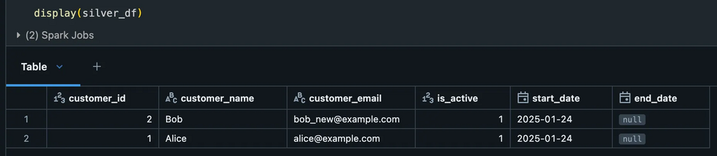
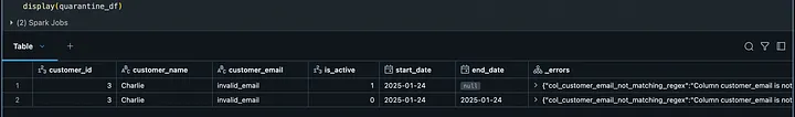
Once your custom data quality rules have been defined and validated, the next step is to apply them to your input data. The DQEngine facilitates this by splitting your dataset into two categories:

Silver Data: Records that meet all quality expectations.
Quarantined Data: Records that fail one or more quality checks.

This approach allows you to separate valid and invalid data for further inspection and remediation. The valid records can proceed to downstream processes, while the quarantined records can be analyzed to determine the cause of failure (e.g., missing values, incorrect formats).

Here’s how you can apply the rules and generate the results:

# Create a DQEngine instance with the WorkspaceClient
dq_engine = DQEngine(WorkspaceClient())

# Apply quality checks and split the DataFrame into silver and quarantine DataFrames
silver_df, quarantine_df = dq_engine.apply_checks_by_metadata_and_split(input_df_1, checks_custom)

Quarantined data – Not matching the rules

Summary

In essence, data quality is no longer just an IT concern; it’s a fundamental business imperative. In today’s complex and competitive landscape, the success of an organization hinges on its ability to leverage high-quality, trusted data for every strategic and operational decision.

A Data Quality Framework (DQX) helps organizations:

Establish clear quality standards
Implement automated checks
Track and resolve issues
Ensure trust in data

https://databrickslabs.github.io/dqx/docs/motivation

https://medium.com/@nivethanvenkat28/revolutionizing-data-quality-checks-using-databricks-dqx-f2a49d83c3c6

Leveraging Microsoft Graph API for SharePoint Manipulation with Azure Data Factory or Synapse Analytics

This article will discuss a new approach for Azure Data Factory (ADF) or Synapse Analytics (ASA) to leverage the Microsoft Graph API for accessing and integrating with various Microsoft 365 services and data. Examples include ADF downloading files from SharePoint (SPO) to Azure Data Lake Storage (ADLS), creating folders in SharePoint libraries, and moving files between SharePoint folders.

We’ve previously discussed using Azure Data Factory (ADF) or Synapse Analytics (ASA) to download files from SharePoint to Azure Data Lake Storage (ADLS) Gen2. Specifically, we explored a metadata-driven approach for incrementally copying data from SharePoint Online to ADLS Gen2.

I recently received reports indicating that our previous method for downloading files from their SharePoint Online (SPO) environment is no longer working. Upon investigation, I confirmed that changes to the configuration of some SharePoint sites prevent the standard download solution from functioning.

What is Microsoft Graph API.

The Microsoft Graph API is a unified RESTful web API provided by Microsoft that allows developers to access and integrate with a wide range of Microsoft 365 services and data. This includes data from:

Azure Active Directory (Entra ID)
Outlook (Mail, Calendar, Contacts)
OneDrive and SharePoint
Teams
Excel
Planner
Intune
To Do, and many others.

Scenario

At Mainri Corporation, colleagues upload files to a designated folder on their SharePoint site. As part of their data centralization process, files from a shared SharePoint Online folder named “Current” are copied to ADLS. Once the copy is successful, these files are then relocated from the “Current” folder to an “Archive” folder within the same SPO Library.

For this purpose, let’s utilize the mainri SharePoint Online (SPO) site, ‘IT-BA-site’ (also known as ‘IT Business Partners’), along with its dummy library and folders. The library’s name is ‘Finance’.

There are multiple folders under the Finance Library, colleagues upload file to:
Finance/Business Requests/AR Aging Report/Current.
The Archive folder is: Finance/Business Requests/AR Aging Report/Archive .

Prerequisites:

An Azure AD Application (AAD) Registration with Microsoft Graph API permissions.

Because SharePoint is a protected Microsoft 365 service, ADF cannot access it directly. So you:

Register an AAD App
Assign it permission to read SharePoint files (Sites.Read.All, Files.Read.All)
Use the AAD App credentials (client ID, secret, tenant ID) to obtain an access token
Pass that token to Microsoft Graph API from ADF pipelines (using Web Activity + HTTP Binary Dataset)

Register an Azure Active Directory Application (AAD App) in Azure

Go to Azure Portal > Azure Active Directory > App registrations.
Click “New registration”.
- Name: ADF-GraphAPI-App
- Supported account types: Single tenant.
Click Register.

we want to get:

Client ID: Unique ID of your app — used in all API calls
Tenant ID: Your Azure AD directory ID
Client Secret: Password-like value — proves app identity
Permissions: Defines what APIs the app is allowed to access

Grant Graph API Permissions

Go to the API permissions tab.

Click “Add a permission” > Microsoft Graph > Application permissions.

Add these (at minimum):

Sites.Read.All – to read SharePoint site content.
Files.Read.All – to read files in document libraries.

Click “Grant admin consent” to enable these permissions.

Solution

The ADF major steps and activities are:

Register an Azure AD Application (if not using Managed Identity), Grant the application the necessary Microsoft Graph API permissions, specifically Sites.Selected.

Enable Managed Identity for your ADF (Recommended), Grant the ADF’s managed identity the necessary Microsoft Graph API permissions, specifically Sites.Selected. Enable Managed Identity for your ADF (Recommended), Grant the ADF’s managed identity the necessary Microsoft Graph API permissions, specifically Sites.Selected.

Create a HTTP Linked Service in ADF,

Base URL:
https://graph.microsoft.com/v1.0

Web Activity to get an access token
URL: https://login.microsoftonline.com/<your_tenant_id>/oauth2/token
Method: POST 

Body: (for Service Principal authentication)
JSON
{
 "grant_type": "client_credentials",
 "client_id": "<your_application_id>",
 "client_secret": "<your_client_secret>",
 "resource": "https://graph.microsoft.com"
}

Authentication: None Headers:Content-Type: application/x-www-form-urlencoded

Web Activity to get the Site ID
URL:https://graph.microsoft.com/v1.0/sites/<your_sharepoint_domain>:/sites/<your_site_relative_path>(e.g., https://mainri.sharepoint.com:/sites/finance) 

Method: GET 

Authentication: none

header: "Authorization" 
@concat('Bearer ', activity('<your_get_token_activity_name>').output.access_token).

Web Activity to list the drives (document libraries)

URL: @concat('https://graph.microsoft.com/v1.0/sites/', activity('<your_get_site_id_activity_name>').output.id, '/drives')
Method: GET

Authentication: none

header: "Authorization" 
@concat('Bearer ', activity('<your_get_token_activity_name>').output.access_token).

Web Activity (or ForEach Activity with a nested Web Activity) to list the items (files and folders) in a specific drive/folder:

URL: @concat('https://graph.microsoft.com/v1.0/drives/', '<your_drive_id>', '/items/<your_folder_id>/children') (You might need to iterate through folders recursively if you have nested structures).

Method: GET

Authentication: none

header: "Authorization" 
@concat('Bearer ', activity('<your_get_token_activity_name>').output.access_token).

Copy Activity to download the file content

Source: HTTP Binary
Relative URL: @item()['@microsoft.graph.downloadUrl']
method: GET

Sink: Configure a sink to your desired destination (e.g., Azure Blob Storage, Azure Data Lake Storage). Choose a suitable format (Binary for files as-is).

Finally, Web Activity move processed file to Archive area.

URL: https://graph.microsoft.com/v1.0/drives/<your_drive_id>/items/<your_file_item_id>

Method; PATCH

Body:
@json(
concat(
' { "parentRefence": {'
, ' "id":" '
, activity('Create_rundate_folder_under_archive').output.id
, ' "}}'
))

Step 1: Get Client Secret from Azure Key Vault

Web activity
purpose: get client secret that saves in Azure Key Vault.

Url: @{concat(
         pipeline().parameters.pl_par_KeyVault_URL
        , '/secrets/'
        , pipeline().parameters.pl_par_keyVault_SecretsName
        , '?api-version=7.0'
)}

Method: Get

Step 2: Get SPO access Bearer Token

Web activity
purpose: all Graph API have to use the Bearer access token

URL: 
@concat(
    'https://login.microsoftonline.com/'
    , pipeline().parameters.pl_par_Tenant_id
    , '/oauth2/v2.0/token'
)

Method: POST

Body: 
@concat(
  'client_id=', pipeline().parameters.pl_par_Client_id,
  '&client_secret=', activity('Get_Client_Secret').output.value,
  '&grant_type=client_credentials',
  '&scope=https://graph.microsoft.com/.default'
)

Header: Content-Type : application/x-www-form-urlencoded

The response has expires_in and ext_expires_in

expires_in: This tells you how many seconds the access token is valid for — in your case, 3599 seconds (which is just under 1 hour). After this time, the token will expire and cannot be used to call the Graph API anymore.

ext_expires_in: This is the extended expiry time. It represents how long the token can still be accepted by some Microsoft services (under specific circumstances) after it technically expires. This allows some apps to use the token slightly longer depending on how token caching and refresh policies are handled.

For production apps, you should always implement token refresh using the refresh token before expires_in hits zero.

Save the token in a variable, as we will use it in subsequent activities.

Set variable activity
Purpose: for following activities conveniences, save it in a variable.

@activity('GetBearerToken').output.access_token

Step 3: Get SPO site ID via Graph API by use Bearer Token

Sometime your SharePoint / MS 365 administrator may give you SiteID. If you do not have it, you can do this way to get it.

Web activity
purpose: We will first obtain the “site ID,” a key value used for all subsequent API calls.

URL:
@concat('https://graph.microsoft.com/v1.0/sites/'
, pipeline().parameters.pl_par_Tenant_name
,'.sharepoint.com:/sites/'
, pipeline().parameters.pl_par_SPO_site
)

Method: GET

Header: 
Authorization
@concat('Bearer ',activity('GetBearerToken').output.access_token)

output segments:
{ ….
“id”: “mainri.sharepoint.com,73751907-6e2b-4228-abcd-3c321f3e00ec,bee66b00-7233-9876-5432-2f0c059ec551″,
….}

from the output, we can see that ID has 3 partitions. the entire 3-part string is the site ID. It is a composite of:

hostname (e.g., mainri.sharepoint.com)
site collection ID (a GUID)
site ID (another GUID)

Step 4: Get SPO Full Drivers list via Graph API by use Bearer Token

“Driver” also known as Library.

Web activity
purpose: Since there are multiple Drivers/Libraries in the SPO, now we list out all Drivers/Libraries; find out the one that we are interested in – Finance.

Url:
 @concat('https://graph.microsoft.com/v1.0/sites/'
, activity('GetSiteId').output.id
, '/drives')

Method: GET

Header: Authorization: @concat('Bearer ',activity('GetBearerToken').output.access_token)

Step 5: Filter out our interested Library “Finance” via Graph API by use Bearer Token

Filter Activity
Purpose: Find out the Finance’s ID.
Since there are multiple drivers/Libraries in the SPO, we are interested in the “Finance” only

Items:@activity('GetFullDrives').output.value
Condition: @equals(item().name, 'Finance')

Output Segments

Save the DriverID/LibraryID in a variable.

We will use the LibraryID/DriverID in the following activities, so save it for convenience.

Step 6: Use the Bearer Token with the Graph API to retrieve a list of subfolders in the Finance library’s root.

Web Activity
Purpose: Navigate to the ‘Business Request’ folder in the Finance library’s sub-folders and retrieve its ID.

URL:
@concat('https://graph.microsoft.com/v1.0/drives/'
, activity('FilterFinance').output.value[0].id
, '/root/children')

Method: GET

Header: Authorization 
@concat('Bearer ',activity('GetBearerToken').output.access_token)

Output segment

Step 7: Find the ‘Business Request’ sub-folder under ‘Finance’.

Filter activity
Purpose: Find out folder “Business Request” ID

Items: @activity('Get_FinanceRoot').output.value
Condition: @equals(item().name, 'Business Requests')

output segments

Step 8: Get “Business Request” child items via Graph API

Check the sub-folders within ‘Business Request’ and identify the one titled ‘AR Aging Report’, as that is our focus

Web Activity
Purpose: Get ‘Business Request’ child items using Graph API.

URL:
@concat('https://graph.microsoft.com/v1.0/drives/'
, activity('FilterFinance').output.value[0].id
, '/items/'
, activity('FilterBusinessRequest').output.value[0].id
, '/children'
)

Method: GET

Header:
Authorization: @concat('Bearer ',activity('GetBearerToken').output.access_token)

output segments

Step 9: Filter out sub-folder “AR Aging Report” from Business Request via Graph API

Filter Activity
Purpose: Maybe, there are multiple child items under this folder. We are interested in the “AR Aging Report” and its ID only.

Items: @activity('GetBusinessRequests_Children').output.value
Condition: @equals(item().name, 'AR Aging Report')

output segment

Step 10: Get “AR Aging Report” child items list

Web Activity
Purpose: We require the folder IDs for the “Current” folder (where colleagues upload files) and the “Archive” folder (for saving processed data), as indicated by the business, to continue.
— “Current” for colleagues uploading files to here
— “Archive” for saving processed files

URL:
@concat('https://graph.microsoft.com/v1.0/drives/'
, activity('FilterFinance').output.value[0].id
, '/items/'
, activity('Filter_AR_Aging_Report').output.value[0].id
, '/children'
)

Method: GET

Header:
Authorization : @concat('Bearer ',activity('GetBearerToken').output.access_token)

output segments

Step 11: Find the ‘Current’ folder under ‘AR Aging Report’

Filter Activity
Purpose: Find out the “Current” folder that saves uploaded files

Items: @activity('Get AR Aging Children').output.value
Condition: @equals(item().name, 'Current')

output segments

Save the Current folder ID in variable

for following activities convenience, save the “Current” folder ID in a variable.

Value: @activity('Filter_Current').output.value[0].id

Step 12: Obtain a list of all files within the ‘Current’ folder.

Web Activity
Purpose: Retrieve a list of files from the ‘Current’ folder to be copied to ADLS.

URL:
@concat('https://graph.microsoft.com/v1.0/drives/'
, activity('FilterFinance').output.value[0].id
, '/items/'
, activity('Filter_Current').output.value[0].id
, '/children'
)

Method: GET

Header: Authorization: @concat('Bearer ',activity('GetBearerToken').output.access_token)

Step 13: Check if today’s folder exists.

If condition Activity
Purpose: To check if a folder for today’s date (2025-05-10) already exists and determine if a new folder needs to be created for today’s archiving.

Expression:
@greater(
    length(activity('Get_Current_Files').output.value) 
    ,1
)

Within the IF-Condition activity “True” activity, there more actions we take.

Since new files are in ‘Current’, we will now COPY and ARCHIVE them.

Find out “Archive” folder, then get the Archive folder ID
List out all child items under “Archive” folder
Run ‘pl_child_L1_chk_rundate_today_exists’ to see if ‘rundate=2025-05-12’ exists. If so, skip creation; if not, create ‘rundate=2025-05-12’ under ‘Archive’..
Get all items in ‘Archive’ and identify the ID of the ‘rundate=2025-05-13’ folder.
Then, run ‘pl_child_L1_copy_archive’ to transfer SPO data to ADLS and archive ‘current’ to ‘Archive/rundate=2025-05-12’.

Begin implementing the actions outlined above.

We begin the process by checking the ‘Current’ folder to identify any files for copying. It’s important to note that this folder might not contain any files at this time.

Step 14: Inside the ‘chk-has-files’ IF-Condition activity, find the ID of ‘Archive’ using a filter.

Filter activity
Purpose: Find “Archive” ID

Items: @activity('Get AR Aging Children').output.value
Condition: @equals(item().name, 'Archive')

Output segments

Step 15: Get Archive’s child items list

Web Activity
Purposes: Check the sub-folders in ‘Archive’ for ‘rundate=2025-05-13‘ to determine if creation is needed.

URL:
@concat('https://graph.microsoft.com/v1.0/drives/'
, activity('FilterFinance').output.value[0].id
, '/items/'
, activity('Filter_Archive').output.value[0].id
, '/children'
)

Method: GET

Header:
Authorization: @concat('Bearer ',activity('GetBearerToken').output.access_token)

Above steps, we have successfully find out all we need:

SiteID
Driver/Library ID
sub-folder(s) ID

We will now create a sub-folder under “archive” with the following naming pattern:
rundate=2024-09-28

“Archive” folder looks:
../Archive/rundate=2024-09-28
…..
../Archive/rundate=2024-11-30
….
etc.

Processed files are archived in sub-folders named by their processing date.
../Archive/rundate=2024-09-28/file1.csv
../Archive/rundate=2024-09-28/file2.xlsx
…
etc.

The Microsoft Graph API will return an error if we attempt to create a folder that already exists. Therefore, we must first verify the folder’s existence before attempting to create it.

As part of today’s data ingestion from SPO to ADLS (May 13, 2025), we need to determine if an archive sub-folder for today’s date already exists. We achieve this by listing the contents of the ‘Archive’ folder and checking for a sub-folder named ‘rundate=2025-05-13‘. If this sub-folder is found, we proceed with the next steps. If it’s not found, we will create a new sub-folder named ‘rundate=2025-05-13‘ within the ‘Archive’ location.

Step 16: Identify the folder named ‘rundate=<<Today Date>>’

Filter activity
Purpose: Verifying the existence of ‘rundate=2025-05-10‘ to determine if today’s archive folder needs creation.

Items: @activity('Get Archive Children').output.value
Condition: @equals(item().name, 
concat(
    'rundate='
    , formatDateTime(convertTimeZone(utcNow(),'UTC' ,'Eastern Standard Time' ),'yyyy-MM-dd')
    )
)

Output segments

(we can see the today’s does not exist.)

Within the IF-Condition activity, if the check for today’s folder returns false (meaning it doesn’t exist), we will proceed to create a new folder named ‘rundate=2025-05-10‘.

Step 17: Execute Child pipeline pl_child_L1_chk_rundate_today_exists

Execute Activity
Purposes: check if rundate=<<Today date>> sub-folder exists or not. If it does not exists, create.

Pass parameters to Child Pipeline:
> child_para_Filter_Archive_rundate_today   ARRAY   @activity('Get Archive Children').output.value
> child_para_bearer_token    string   @variables('var_Bearer_Token')
> child_para_rundate    string   @variables('var_rundate')
> child_para_FinanceID   string   @variables('var_financeID')
> child_para_archiveID   string   @variables('var_ArchiveID')

Step 18: Check if “rundate=<<Today date>>” exists or not

In the Child Pipeline: pl_child_L1_chk_rundate_today_exists

If-Condition Activity
Purpose: Verify the existence of the ‘rundate=<<Today Date>>‘ sub-folder; create it if it doesn’t exist.

Child pipeline parameters:
> child_para_Filter_Archive_rundate_today    ARRAY 
> child_para_bearer_token   string
> child_para_rundate   string
> child_para_FinanceID   string
> child_para_archiveID   string

Step 19: Create a new folder in “Archive” via Graph API

Inside IF-Condition activity, TRUE

Web Activity
Purpose: create a new folder name it rundate=<today date>
e.g. rundate=2024-05-10

URL:
@concat('https://graph.microsoft.com/v1.0/drives/'
, activity('FilterFinance').output.value[0].id
, '/items/'
,  variables('var_ArchiveID')
, '/children'
)

Method: POST

Body:
@json(
concat(
    '{"name": "', variables('var_rundate'), '",  "folder":{} }'
))

Header:
Authorization: @concat('Bearer ',activity('GetBearerToken').output.access_token)

Content-Type: application/json

output segments

After creating the new folder, we will extract its ID. This ID will then be stored in a variable for use during the “Archiving” process.

Step 20: Get “Archive” folder child Items Again

As the ‘rundate=2024-05-12‘ folder could have been created either in the current pipeline run (during a previous step) or in an earlier execution today, we are re-retrieving the child items of the ‘Archive’ folder to ensure we have the most up-to-date ID.

In the Main pipeline IF-Condition TRUE active.

Web Activity

URL: 
@concat('https://graph.microsoft.com/v1.0/drives/'
, activity('FilterFinance').output.value[0].id
, '/items/'
, activity('Filter_Archive').output.value[0].id
, '/children'
)

Method: GET

Header:
Authorization:  @concat('Bearer ',activity('GetBearerToken').output.access_token)

output similar to Step 15: get Archive’s child items list

Step 21: Find the ‘rundate=2024-05-12‘ folder in Archive and get its ID agin.

Within main pipeline, IF-Condition TRUE active.

Filter Activity
Purpose: Retrieve the ID of the sub-folder named “rundate=2024-05-12“.

Items: @activity('Get Archive Children').output.value
Condition: @equals(item().name, 
variables('var_rundate')
)

output similar to Step 16: Filter out rundate today folder

Save rundate=<<Today Date>> ID in a variable

Next, we retrieve the files from the ‘Current’ SPO folder for copying to ADLS.

Step 22: Execute child pipeline pl_child_L1_copy_archive

In the Main pipeline, if-Condition TRUE activity,

Execute Activity
Purpose: Implement the process to copy files from SPO to ADLS and archive processed files from the “Current” folder in SPO to the “Archive” folder in SPO.

Pass parameters to child pipeline pl_child_L1_copy_archive:
> child_para_tar_path   string   @pipeline().parameters.pl_tar_path
> child_para_version   string   @pipeline().parameters.pl_par_version
> child_para_item   string   @variables('var_current_files_list')
> child_para_Bearer_Token   string   @variables('var_Bearer_Token')
> child_para_rundateTodayID   string   @variables('var_rundate_today_FolderID')
> child_para_FinanceID   string   @variables('var_financeID')

Execute child pipeline pl_child_L1_copy_archive

In the child pipeline pl_child_L1_copy_archive

ForEach activity
Purpose: Iterate through each item in the file list.

Items: @pipeline().parameters.child_para_item

The ForEach loop will iterate through each file, performing the following actions: copying the file to Azure Data Lake Storage and subsequently moving the processed file to the ‘Archive’ folder.

Step 23: Copy file to ADLS

Copy activity
purpose: copy file to ADLS one by one

Linked Service:

HTTP linked service, use Anonymous.

Source DataSet:

HTTP Binary dataset,

Sink Dataset

Azure Data Lake Storage Gen 2, Binary

Linked Services

Azure Data Lake Storage Gen 2

Sink dataset parameters:
ds_par_dst_path   string
ds_par_dst_fname   string

Step 24: Move processed file to “Archive” Folder

In the child pipeline pl_child_L1_copy_archive

Web Activity
Prupose: Move processed file from “Currrent” folder to “Archive” area.

URL:
@concat(
    'https://graph.microsoft.com/v1.0/drives/'
    , pipeline().parameters.child_para_FinanceID
    ,'/items/'
    , item().id
)

Method: PATCH

Body:
@json(
concat(
'{ "parentReference": {'
    , '"id": "'
    , activity('Create_rundate_folder_under_archive').output.id
    , '"}}'
))

Headers:
Authorization: @concat('Bearer ',activity('GetBearerToken').output.access_token)

Summary

The pipeline includes checks for folder existence to avoid redundant creation, especially in scenarios where the pipeline might be re-run. The IDs of relevant folders (“Archive” and the date-specific sub-folders) are retrieved dynamically throughout the process using filtering and list operations.

In essence, this pipeline automates the process of taking newly uploaded files, transferring them to ADLS, and organizing them within an archive structure based on the date of processing.

Register an Azure AD Application (if not using Managed Identity), Grant the application the necessary Microsoft Graph API permissions, specifically Sites.Selected.
Enable Managed Identity for your ADF (Recommended), Grant the ADF’s managed identity the necessary Microsoft Graph API permissions, specifically Sites.Selected. Enable Managed Identity for your ADF (Recommended), Grant the ADF’s managed identity the necessary Microsoft Graph API permissions, specifically Sites.Selected.
Create a HTTP Linked Service in ADF, Base URL: https://graph.microsoft.com/v1.0
Web Activity to get an access token
URL:https://login.microsoftonline.com/<your_tenant_id>/oauth2/tokenMethod: POST
Body: (for Service Principal authentication)
JSON
{ “grant_type”: “client_credentials”,
“client_id”: “<your_application_id>”,
“client_secret”: “<your_client_secret>”,
“resource”: “https://graph.microsoft.com”
}
Authentication: None
Headers: Content-Type: application/x-www-form-urlencoded
get the Site ID
Web Activity to get the Site ID
URL:https://graph.microsoft.com/v1.0/sites/<your_sharepoint_domain>:/sites/<your_site_relative_path>
(e.g., https://mainri.sharepoint.com:/sites/finance)
Method: GET
Authentication: none
header: “Authorization”
@concat('Bearer ', activity('<your_get_token_activity_name>').output.access_token).
Web Activity to list the drives (document libraries)
URL: @concat('https://graph.microsoft.com/v1.0/sites/', activity('<your_get_site_id_activity_name>').output.id, '/drives')
Method: GET
Authentication: none
header: “Authorization”
@concat('Bearer ', activity('<your_get_token_activity_name>').output.access_token).
Web Activity (or ForEach Activity with a nested Web Activity) to list the items (files and folders) in a specific drive/folder:
URL: @concat('https://graph.microsoft.com/v1.0/drives/', '<your_drive_id>', '/items/<your_folder_id>/children') (You might need to iterate through folders recursively if you have nested structures).
Method: GET
Authentication: none
header: “Authorization”
@concat('Bearer ', activity('<your_get_token_activity_name>').output.access_token).
Copy Activity to download the file content
Source: HTTP Binary
Relative URL: @item()['@microsoft.graph.downloadUrl']
method: GET
Sink: Configure a sink to your desired destination (e.g., Azure Blob Storage, Azure Data Lake Storage). Choose a suitable format (Binary for files as-is).
Finally, Web Activity move processed file to Archive area.
URl: https://graph.microsoft.com/v1.0/drives/<your_drive_id>/items/<your_file_item_id>
Method; PATCH
Body:
@json(concat(
‘ { “parentRefence”: {‘, ‘ “id”:” ‘
, activity(‘Create_rundate_folder_under_archive’).output.id, ‘ “}}’))

Please do not hesitate to contact me if you have any questions at William . chen @ mainri.ca

(remove all space from the email account 😊)

Microsoft Fabric vs Databricks vs Synapse

Architecture

Main Use Cases

V-Order

Z-Order

Liquid Clustering

Ultra-short memory trick

The Best Setup for 2026

General terms

Capacity

Direct Lake

Experience

Experiment

IQ

Item

Lakehouse

Liquid Clustering

OneLake

Shortcut

V-order

Workload / Experience

Workspace

What is Fabic?

Why use Microsoft Fabric?

What can Microsoft Fabric do?

Components of Fabric

Step-by-Step: Getting Started

Step 1: Create a Workspace

Step 2: The Lakehouse (Bronze)

Step 3: Data Pipeline (Ingestion

Step 4: Notebook (Silver/Gold)

Step 5: Power BI (Visualization)

log levels in Python

Logging Level Quick Reference

Logging basic configuration

simple logging example

Log Rotation (Daily Files)

Logging to Unity Catalog Volume (BEST PRACTICE)

Databricks ETL Logging Template (Production-Ready)

Features

1. Create the logger (ready for copy & paste)

“File Version”

Unity Catalog Volume version

2. Use the logger inside your ETL

Resulting log file (example)

Best Practices for Logging in Python

Conclusion

Azure Data Factory+

Azure Databricks / Delta / Unity Catalog / Lakehouse+

Azure Synapse Analytics +

SQL+

1. Shared Lock (S)

2. Exclusive Lock (X)

3. Update Lock (U) (SQL Server specific)

4. Intention Locks (IS, IX, SIX)

5. Row / Page / Table Locks

A: In SQL Server: Enable Deadlock Graph Capture

B: Interpret the Deadlock Graph

C. Identify

KQL+

Micorsoft Fabric+

Power BI+

Purview+

Sentinel+

Why is it Important?

Key Features and Syntax with Examples

1. Headers (for Structure)

Title (H1)

Section 1 (H2)

Subsection 1.1 (H3)

This is a H4 Header

2. Emphasis (Bold and Italic)

3. Lists (Ordered and Unordered)

Unordered List:

Ordered List:

4. Links and Images

link

Image

5. Tables

6. Code Syntax Highlighting (A Powerful Feature)