alias(), asc(), desc(), cast(), filter(), where(), like() functions

alias ()

alias () is used to assign a temporary name or “alias” to a DataFrame, column, or table, which can be used for reference in further operations

# for dataframe: 
df1 = df.alias("df1")
df1.show()
==output==
+---+---+
| id|age|
+---+---+
|  1| 25|
|  2| 12|
|  3| 40|
+---+---+

caution: df.alias(“newName”) will not generate new dataframe,

# for column: 
df.select(df.id.alias("new_ID")).show()
df.select(df["id"].alias("new_ID")).show()
df.select(col("id").alias("new_ID")).show()
==output==
+------+
|new_ID|
+------+
|     1|
|     2|
|     3|
+------+

asc(), desc ()

asc (): ascending order when sorting the rows of a DataFrame by one or more columns.

sample df
+---+---+
| id|age|
+---+---+
|  1| 25|
|  2| 12|
|  3| 40|
+---+---+
from pyspark.sql.functions import asc
df.orderBy(asc("age")).show()
==output==
+---+---+
| id|age|
+---+---+
|  2| 12|
|  1| 25|
|  3| 40|
+---+---+

desc (): descending order when sorting the rows of a DataFrame by one or more columns.

from pyspark.sql.functions import desc
df.orderBy(desc("age")).show()
==output==
+---+---+
| id|age|
+---+---+
|  3| 40|
|  1| 25|
|  2| 12|
+---+---+

cast ()

df[“column_name”].cast(“new_data_type”)

This can be a string representing the data type (e.g., "int", "double", "string", etc.) or a PySpark DataType object (like IntegerType(), StringType(), FloatType(), etc.).

Common Data Types:

  • IntegerType(), "int": For integer values.
  • DoubleType(), "double": For double (floating-point) values.
  • FloatType(), "float": For floating-point numbers.
  • StringType(), "string": For text or string values.
  • DateType(), "date": For date values.
  • TimestampType(), "timestamp": For timestamps.
  • BooleanType(), "boolean": For boolean values (true/false).
sample dataframe
+---+---+
| id|age|
+---+---+
|  1| 25|
|  2| 12|
|  3| 40|
+---+---+

df.printSchema()
root
 |-- id: long (nullable = true)
 |-- age: long (nullable = true)
from pyspark.sql.functions import col

# Cast a string column to integer
df1 = df.withColumn("age_int", col("age").cast("int"))
df1.printSchema()

==output==
root
 |-- id: long (nullable = true)
 |-- age: long (nullable = true)
 |-- age_int: integer (nullable = true)


# Cast 'id' from long to string and 'age' from long to double
df_casted = df.withColumn("id", col("id").cast("int")) \
              .withColumn("age", col("age").cast("double"))
df_casted.show()              
df_casted.printSchema()  

==output==
+---+----+
| id| age|
+---+----+
|  1|25.0|
|  2|12.0|
|  3|40.0|
+---+----+

root
 |-- id: string (nullable = true)
 |-- age: double (nullable = true)

filter (), where (),

filter () or where () function is used to filter rows from a DataFrame based on a condition or set of conditions. It works similarly to SQL’s WHERE clause,

df.filter(condition)
df.where(condition)

Condition (for ‘filter’)

  • & (AND)
  • | (OR)
  • ~ (NOT)
  • == (EQUAL)

all “filter” can change to “where”, vice versa.

sample dataframe
+------+---+-------+
|  Name|Age|Salary|
+------+---+-------+
| Alice| 30|  50000|
|   Bob| 25|  30000|
|Alicia| 40|  80000|
|   Ann| 32|  35000|
+------+---+-------+

# Filter rows where age is greater than 30 AND salary is greater than 50000
df.filter((df["age"] > 30) & (df["salary"] > 50000))
df.where((df["age"] > 30) & (df["salary"] > 50000))

+------+---+------+
|  Name|Age|Salary|
+------+---+------+
|Alicia| 40| 80000|
+------+---+------+

# Filter rows where age is less than 25 OR salary is less than 40000
df.filter((df["age"] < 25) | (df["salary"] < 40000))
df.where((df["age"] < 25) | (df["salary"] < 40000))

+----+---+------+
|Name|Age|Salary|
+----+---+------+
| Bob| 25| 30000|
| Ann| 32| 35000|
+----+---+------+

like ()


like() function is used to perform pattern matching on string columns, similar to the SQL LIKE operator

df.filter(df[“column_name”].like(“pattern”))

Pattern

  • %: Represents any sequence of characters.
  • _: Represents a single character.

pattern is case sensitive.

sample dataframe
+------+---+
|  Name|Age|
+------+---+
| Alice| 30|
|   Bob| 25|
|Alicia| 28|
|   Ann| 32|
+------+---+


# Filtering names that start with 'Al'
df.filter(df["Name"].like("Al%")).show()

+------+---+
|  Name|Age|
+------+---+
| Alice| 30|
|Alicia| 28|
+------+---+

# Filtering names that end with 'n'
df.filter(df["Name"].like("%n")).show()

+----+---+
|Name|Age|
+----+---+
| Ann| 32|
+----+---+

# Filtering names that contain 'li'
df.filter(df["Name"].like("%li%")).show()

+------+---+
|  Name|Age|
+------+---+
| Alice| 30|
|Alicia| 28|
+------+---+

# Filtering names where the second letter is 'l'
df.filter(df["Name"].like("A_l%")).show()

+----+---+
|Name|Age|
+----+---+
+----+---+
nothing found in this pattern 

condition: when (), otherwise (), expr()

if - else - " logic implementing

In PySpark, there isn’t an explicit “if-else" statement construct like in regular Python. Instead, PySpark provides several ways to implement conditional logic using functions such as when (), otherwise (), withColumn(), expr (), UDF etc.

using when (), expr() look at following sections. now focus on UDF to implement “if — then — else –” logic”.

from pyspark.sql.functions import udf
from pyspark.sql.types import StringType

# Define a Python function for age classification
def classify_age(age):
    if age >= 18:
        return 'Adult'
    else:
        return 'Minor'

# Register the function as a UDF
classify_age_udf = udf(classify_age, StringType())

# Create the DataFrame
data = [(1, 25), (2, 12), (3, 40)]
df = spark.createDataFrame(data, ["id", "age"])
+---+---+
| id|age|
+---+---+
|  1| 25|
|  2| 12|
|  3| 40|
+---+---+

# Apply the UDF to create a new column with the if-else logic
df = df.withColumn("age_group", classify_age_udf(df["age"]))

df.show()
+---+---+---------+
| id|age|age_group|
+---+---+---------+
|  1| 25|    Adult|
|  2| 12|    Minor|
|  3| 40|    Adult|
+---+---+---------+

In this example:

  • The function classify_age behaves like a Python if-else statement.
  • The UDF (classify_age_udf) applies this logic to the DataFrame.

when (), otherwise ()

when function in PySpark is used for conditional expressions, similar to SQL’s CASE WHEN clause.

Syntax

from pyspark.sql.functions import when
when(condition, value).otherwise(default_value)

Parameters

  • condition: A condition that returns a boolean (True/False). If this condition is true, the function will return the specified value.
  • value: The value to return when the condition is true.
  • otherwise(default_value): An optional method that specifies the default value to return when the condition is false.

sample dataframe

+—+—–+
| id|score|
+—+—–+
| 1| 92|
| 2| 85|
| 3| 98|
| 4| 59|
+—+—–+

from pyspark.sql.functions import when, col

# Multiple Conditions with AND/OR/NOT Logic
# AND : &
# OR : |
# NOT : ~
df = df.withColumn("grade", 
        when(col("score") >= 90, "A") 
        .when((col("score") >= 80) & (col("score") < 90), "B") 
        .when((col("score") >= 70) & (col("score") < 80), "C") 
        .otherwise("F"))
==output==
+---+-----+-----+
| id|score|grade|
+---+-----+-----+
|  1|   92|    A|
|  2|   85|    B|
|  3|   98|    A|
|  4|   59|    F|
+---+-----+-----+

expr ()

The expr () function allows you to use SQL expressions as a part of the DataFrame transformation logic.

Syntax

expr ()
from pyspark.sql.functions import expr
expr(sql_expression)

Parameters:

  • sql_expression: A string containing a SQL-like expression to be applied to the DataFrame. It can contain any valid SQL operations, such as arithmetic operations, column references, conditional logic, or function calls.

sample dataframe

+—+—–+
| id | value|
+—+—–+
| 1| 10|
| 2| 20|
| 3| 30|
+—+—–+

from pyspark.sql.functions import expr

# Use expr() to apply arithmetic operations
df = df.withColumn("double_value", expr("value * 2"))

==output==
+---+-----+------------+
| id|value|double_value|
+---+-----+------------+
|  1|   10|          20|
|  2|   20|          40|
|  3|   30|          60|
+---+-----+------------+

# Apply conditional logic using expr()
df = df.withColumn("category", expr("CASE WHEN value >= 20 THEN 'High' ELSE 'Low' END"))

df.show()
+---+-----+------------+--------+
| id|value|double_value|category|
+---+-----+------------+--------+
|  1|   10|          20|     Low|
|  2|   20|          40|    High|
|  3|   30|          60|    High|
+---+-----+------------+--------+

# Use SQL function CONCAT
df = df.withColumn("full_category", expr("CONCAT(category, '_Category')"))

df.show()
+---+-----+------------+--------+-------------+
| id|value|double_value|category|full_category|
+---+-----+------------+--------+-------------+
|  1|   10|          20|     Low| Low_Category|
|  2|   20|          40|    High|High_Category|
|  3|   30|          60|    High|High_Category|
+---+-----+------------+--------+-------------+

selectExpr ()

The selectExpr() method allows you to directly select columns or apply SQL expressions on multiple columns simultaneously, similar to SQL’s SELECT statement.

Syntax

from pyspark.sql.functions import selectExpr

df.selectExpr(*sql_expressions)

Parameters:

  • sql_expression: A list of SQL-like expressions (as strings) that define how to transform or select columns. Each expression can involve selecting a column, renaming it, applying arithmetic, or adding conditions using SQL syntax.

sample dataframe

+—+—–+
| id | value|
+—+—–+
| 1| 10|
| 2| 20|
| 3| 30|
+—+—–+

from pyspark.sql.functions import selectExpr

# Select specific columns and rename them using selectExpr()
df = df.selectExpr("id", "value * 2 as double_value", "value as original_value")

df.show()

==output==
+---+------------+--------------+
| id|double_value|original_value|
+---+------------+--------------+
|  1|          20|            10|
|  2|          40|            20|
|  3|          60|            30|
+---+------------+--------------+

# Use CASE WHEN to categorize values
df = df.selectExpr("id", "value", "CASE WHEN value >= 20 THEN 'High' ELSE 'Low' END as category")

df.show()
+---+-----+--------+
| id|value|category|
+---+-----+--------+
|  1|   10|     Low|
|  2|   20|    High|
|  3|   30|    High|
+---+-----+--------+

# Apply multiple transformations and expressions
df = df.selectExpr("id", "value", "value * 2 as double_value", "CASE WHEN value >= 20 THEN 'High' ELSE 'Low' END as category")

df.show()
+---+-----+------------+--------+
| id|value|double_value|category|
+---+-----+------------+--------+
|  1|   10|          20|     Low|
|  2|   20|          40|    High|
|  3|   30|          60|    High|
+---+-----+------------+--------+

comparison: expr () and selectExpr ()

Key Differences
expr () is used when you want to apply SQL-like expressions in the middle of a transformation, typically within withColumn() or filter().
selectExpr() is used when you want to apply multiple expressions in a single statement to transform and select columns, much like a SQL SELECT statement.

Featureexpr()selectExpr()
PurposeUsed for applying single SQL expressionsUsed for applying multiple SQL expressions
Typical UsageInside select(), withColumn(), filter()As a standalone method for multiple expressions
Operates OnIndividual column expressionsMultiple expressions at once
FlexibilityAllows complex operations on a single columnSimpler for multiple transformations
Exampledf.select(expr("age + 5").alias("new_age"))df.selectExpr("age + 5 as new_age", "age * 2")
Use CaseFine-grained control of expressions in various transformationsQuickly apply and select multiple expressions as new columns

Conclusion
expr (): Ideal for transforming or adding individual columns using SQL expressions.
selectExpr (): Useful for selecting, renaming, and transforming multiple columns at once using SQL-like syntax.


na.fill ()

na.fill(): Used to replace null values in DataFrames.

Syntax
df.na.fill( {“vaule”:0} )

sample dataframe

data = [(1, 10), (2, 20), (3, 30),(4,None)]
df = spark.createDataFrame(data, [“id”, “value”])
+—+—–+
| id | value|
+—+—–+
| 1 | 10|
| 2 | 20|
| 3 | 30|
| 4 | null|
+—+—–+

caution: in pyspark, “NULL” is None

#Fill null values in a specific column with a default value (e.g., 0)
df = df.na.fill({"value": 0})

df.show()
==output==
+---+-----+
| id|value|
+---+-----+
|  1|   10|
|  2|   20|
|  3|   30|
|  4|    0|
+---+-----+

coalescs ()

coalesce function is used to return the first non-null value among the columns you provide

Syntax

from pyspark.sql.functions import coalesce
coalesce(col1, col2, …, colN)

from pyspark.sql.functions import coalesce

# Return the first non-null value from multiple columns
df = df.withColumn("first_non_null", coalesce(col("column1"), col("column2"), col("column3")))

isin ()

isin function is used to check if a value belongs to a list or set of values.

Syntax
from pyspark.sql.functions import col
col(“column_name”).isin(value1, value2, …, valueN)

sample dataframe

data = [(1, 10), (2, 20), (3, 30),(4,None)]
df = spark.createDataFrame(data, [“id”, “value”])
+—+—–+
| id | value|
+—+—–+
| 1 | 10|
| 2 | 20|
| 3 | 30|
| 4 | null|
+—+—–+

caution: in pyspark, “NULL” is None

from pyspark.sql.functions import col
df = df.withColumn("is_in_list", col("value").isin(18, 25, 30)).show()

df.show()
==output==
+---+-----+----------+
| id|value|is_in_list|
+---+-----+----------+
|  1|   10|     false|
|  2|   20|     false|
|  3|   30|      true|
|  4|    0|     false|
+---+-----+----------+

between ()

The between function allows you to check whether a column’s value falls within a specified range.

Syntax
from pyspark.sql.functions import col
col(“column_name”).between(lower_bound, upper_bound)

sample dataframe

data = [(1, 10), (2, 20), (3, 30),(4,31)]
df = spark.createDataFrame(data, [“id”, “value”])
+—+—–+
| id | value|
+—+—–+
| 1 | 10|
| 2 | 20|
| 3 | 30|
| 4 | 31|
+—+—–+

from pyspark.sql.functions import col
# Check if the value is between 20 and 30
df = df.withColumn("value_between_20_and_30", col("value").between(20, 30)).show()

df.show()
==output==
+---+-----+-----------------------+
| id|value|value_between_20_and_30|
+---+-----+-----------------------+
|  1|   15|                  false|
|  2|   20|                   true|
|  3|   30|                   true|
|  4|   36|                  false|

note: it included boundary value - "20" and "30"

isNull (), isNotNull ()

PySpark provides isNull and isNotNull functions to check for null values in DataFrame columns.

Syntax
col(“column_name”).isNull()
col(“column_name”).isNotNull()

sample dataframe
+—+—-+
| id| age|
+—+—-+
| 1| 15|
| 2|null|
| 3| 45|
+—+—-+

from pyspark.sql.functions import col
# Check if the 'name' column has null values
df = df.withColumn("has_null_name", col("name").isNull())


# Check if the 'age' column has non-null values
df = df.withColumn("has_age", col("age").isNotNull()).show()
==output==
+---+----+--------+
| id| age|has_age |
+---+----+--------+
|  1|  25|   true |
|  2|null|  false |
|  3|  45|   true |
+---+----+--------+

withColumn, select

withColumn()

It’s a “transformation”.
withColumn() add or replace a column_name in a DataFrame. In other words, if “column_name” exists, replace/change the existing column, otherwise, add “column_name” as new column.

Syntax:

from pyspark.sql.functions import col, lit, concat, when, upper, coalesce
df.withColumn(“column_name”, expression)

Key Parameters

  • "column_name": The name of the new or existing column.
  • expression: Any transformation, calculation, or function applied to create or modify the column.
Basic Column Creation (with literal values)

from pyspark.sql.functions import lit
# Add a column with a constant value
df_new = df.withColumn(“New_Column”, lit(100))

===output===
ID Name Grade New_Column
1 Alice null 100
2 Bob B 100
3 Charlie C 100

# Add a new column, no value
df_new = df.withColumn(“New_Column”, lit(None))

===output===
ID Name Grade New_Column
1 Alice null null
2 Bob B null
3 Charlie C null

Arithmetic Operation

from pyspark.sql.functions import col
# Create a new column based on arithmetic operations
df_arithmetic = df.withColumn(“New_ID”, col(“ID”) * 2 + 5)
df_arithmetic.show()
===output===
ID Name Grade New_ID
1 Alice null 7
2 Bob B 9
3 Charlie C 11

Using SQL Function

you can use functions like concat(), substring(), when(), length(), etc.

from pyspark.sql.functions import concat, lit
# Concatenate two columns with a separator
df_concat = df.withColumn(“Full_Description”, concat(col(“Name”), lit(” has ID “), col(“ID”)))

Conditional Logic

Using when() and otherwise() is equivalent to SQL’s CASE WHEN expression.

from pyspark.sql.functions import when

# Add a new column with conditional logic
df_conditional = df.withColumn("Is_Adult", when(col("ID") > 18, "Yes").otherwise("No"))
df_conditional.show()
String Function

You can apply string functions like upper(), lower(), or substring()

from pyspark.sql.functions import upper
# Convert a column to uppercase
df_uppercase = df.withColumn(“Uppercase_Name”, upper(col(“Name”)))
df_uppercase.show()

Type Casting

You can cast a column to a different data type.

Cast the ID column to a string

# Cast the ID column to a string
df_cast = df.withColumn(“ID_as_string”, col(“ID”).cast(“string”))
df_cast.show()

Handling Null Values

create columns that handle null values using coalesce() or fill()

Coalesce:

This function returns the first non-null value among its arguments.

from pyspark.sql.functions import coalesce
# Return non-null value between two columns
df_coalesce = df.withColumn(“NonNullValue”, coalesce(col(“Name”), lit(“Unknown”)))
df_coalesce.show()

Fill Missing Values:

# Replace nulls in a column with a default value
df_fill = df.na.fill({“Name”: “Unknown”})
df_fill.show()

Creating Columns with Complex Expressions

create columns based on more complex expressions or multiple transformations at once.

# Create a column with multiple transformations
df_complex = df.withColumn( “Complex_Column”, concat(upper(col(“Name”)), lit(“_”), col(“ID”).cast(“string”)) )
df_complex.show(truncate=False)

example
from pyspark.sql import SparkSession
from pyspark.sql.functions import col, lit, concat, when, upper, coalesce

# Initialize Spark session
spark = SparkSession.builder.appName("withColumnExample").getOrCreate()

# Create a sample DataFrame
data = [(1, "Alice", None), (2, "Bob", "B"), (3, "Charlie", "C")]
df = spark.createDataFrame(data, ["ID", "Name", "Grade"])

# Perform various transformations using withColumn()
df_transformed = df.withColumn("ID_Multiplied", col("ID") * 10) \
                   .withColumn("Full_Description", concat(upper(col("Name")), lit(" - ID: "), col("ID"))) \
                   .withColumn("Pass_Status", when(col("Grade") == "C", "Pass").otherwise("Fail")) \
                   .withColumn("Non_Null_Grade", coalesce(col("Grade"), lit("N/A"))) \
                   .withColumn("ID_as_String", col("ID").cast("string"))

# Show the result
df_transformed.show(truncate=False)
==output==
ID	Name	Grade	ID_Multiplied	Full_Description	Pass_Status	Non_Null_Grade	ID_as_String
1	Alice	null	10	ALICE - ID: 1	Fail	N/A	1
2	Bob	B	20	BOB - ID: 2	Fail	B	2
3	Charlie	C	30	CHARLIE - ID: 3	Pass	C	3

select ()

select () is used to project (select) a set of columns or expressions from a DataFrame. This function allows you to choose and work with specific columns, create new columns, or apply transformations to the data.

Syntax

DataFrame.select(*cols)

Commonly Used PySpark Functions with select()

  • col(column_name): Refers to a column.
  • alias(new_name): Assigns a new name to a column.
  • lit(value): Adds a literal value.
  • round(column, decimals): Rounds off the values in a column.
  • concat(col1, col2, ...): Concatenates multiple columns.
  • when(condition, value): Adds conditional logic.
Renaming Columns:
df.select(df["column1"].alias("new_column1"), df["column2"]).show()

Using Expressions:
from pyspark.sql import functions as F
df.select(F.col("column1"), F.lit("constant_value"), (F.col("column2") + 10).alias("modified_column2")).show()

Performing Calculations
df.select((df["column1"] * 2).alias("double_column1"), F.round(df["column2"], 2).alias("rounded_column2")).show()

Handling Complex Data Types (Struct, Array, Map):
df.select("struct_column.field_name").show()

Selecting with Wildcards:

While PySpark doesn’t support SQL-like wildcards directly, you can achieve similar functionality using selectExpr (discussed below) or other methods like looping over df.columns.

df.select([c for c in df.columns if “some_pattern” in c]).show()

Using selectExpr ()

df.selectExpr(“column1”, “column2 + 10 as new_column2”).show()

Pyspark: read and write a parquet file

Reading Parquet Files

Syntax

help(spark.read.parquet)


df = spark.read \
    .format("parquet") \
    .option("mergeSchema", "true") \  # Merges schemas of all files (useful when reading from multiple files with different schemas)
    .option("pathGlobFilter", "*.parquet") \  # Read only specific files based on file name patterns
    .option("recursiveFileLookup", "true") \  # Recursively read files from directories and subdirectories
.load("/path/to/parquet/file/or/directory")

Options

  • mergeSchema: When reading Parquet files with different schemas, merge them into a single schema.
    • true (default: false)
  • pathGlobFilter: Allows specifying a file pattern to filter which files to read (e.g., “*.parquet”).
  • recursiveFileLookup: Reads files recursively from subdirectories.
    • true (default: false)
  • modifiedBefore/modifiedAfter: Filter files by modification time. For example:
    .option(“modifiedBefore”, “2023-10-01T12:00:00”)
    .option(“modifiedAfter”, “2023-01-01T12:00:00”)
  • maxFilesPerTrigger: Limits the number of files processed in a single trigger, useful for streaming jobs.
  • schema: Provides the schema of the Parquet file (useful when reading files without inferring schema).

from pyspark.sql.types import StructType, StructField, IntegerType, StringTypeschema = StructType([StructField("id", IntegerType(), True),  StructField("name", StringType(), True)]) 

df = spark.read.schema(schema).parquet("/path/to/parquet")

Path
  • Load All Files in a Directory
    df = spark.read.parquet(“/path/to/directory/”)
  • Load Multiple Files Using Comma-Separated Paths
    df = spark.read.parquet(“/path/to/file1.parquet”, “/path/to/file2.parquet”, “/path/to/file3.parquet”)
  • Using Wildcards (Glob Patterns)
    df = spark.read.parquet(“/path/to/directory/*.parquet”)
  • Using Recursive Lookup for Nested Directories
    df = spark.read.option(“recursiveFileLookup”, “true”).parquet(“/path/to/top/directory”)
  • Load Multiple Parquet Files Based on Conditions
    df = spark.read .option(“modifiedAfter”, “2023-01-01T00:00:00”) .parquet(“/path/to/directory/”)
  • Programmatically Load Multiple Files
    file_paths = [“/path/to/file1.parquet”, “/path/to/file2.parquet”, “/path/to/file3.parquet”]
    df = spark.read.parquet(*file_paths)
  • Load Files from External Storage (e.g., S3, ADLS, etc.)
    df = spark.read.parquet(“s3a://bucket-name/path/to/files/”)

Example


# Reading Parquet files with options
df = spark.read \
    .format("parquet") \
    .option("mergeSchema", "true") \
    .option("recursiveFileLookup", "true") \
    .load("/path/to/parquet/files")

Conclusion

To load multiple Parquet files at once, you can:

  • Load an entire directory.
  • Use wildcard patterns to match multiple files.
  • Recursively load from subdirectories.
  • Programmatically pass a list of file paths. These options help streamline your data ingestion process when dealing with multiple Parquet files in Databricks.

Write to parquet

Syntax


# Writing a Parquet file
df.write \
    .format("parquet") \
    .mode("overwrite") \  # Options: "overwrite", "append", "ignore", "error"
    .option("compression", "snappy") \  # Compression options: none, snappy, gzip, lzo, brotli, etc.
    .option("maxRecordsPerFile", 100000) \  # Max number of records per file
    .option("path", "/path/to/output/directory") \
    .partitionBy("year", "month") \  # Partition the output by specific columns
.save()

Options

compression: .option(“compression”, “snappy”)

Specifies the compression codec to use when writing files.
Options: none, snappy (default), gzip, lzo, brotli, lz4, zstd, etc.

maxRecordsPerFile: .option(“maxRecordsPerFile”, 100000)

Controls the number of records per file when writing.
Default: None (no limit).

saveAsTable: saveAsTable(“parquet_table”)

Saves the DataFrame as a table in the catalog.

Save: save()
path:

Defines the output directory or file path.

mode: mode(“overwrite”)

Specifies the behavior if the output path already exists.

  • overwrite: Overwrites existing data.
  • append: Appends to existing data.
  • ignore: Ignores the write operation if data already exists.
  • error or errorifexists: Throws an error if data already exists (default).
Partition: partitionBy(“year”, “month”)

Partitions the output by specified columns

bucketBy: .bucketBy(10, “id”)

Distributes the data into a fixed number of buckets

df.write \
    .bucketBy(10, "id") \
    .sortBy("name") \
.saveAsTable("parquet_table")

Example


# Writing Parquet files with options
df.write \
    .format("parquet") \
    .mode("overwrite") \
    .option("compression", "gzip") \
    .option("maxRecordsPerFile", 50000) \
    .partitionBy("year", "month") \
    .save("/path/to/output/directory")

writing key considerations:

  • Use mergeSchema if the Parquet files have different schemas, but it may increase overhead.
  • Compression can significantly reduce file size, but it can add some processing time during read and write operations.
  • Partitioning by columns is useful for organizing large datasets and improving query performance.

Pyspark: read, write and flattening complex nested json

Reading JSON Files

Syntax

df = spark.read.option(options).schema(schame).json(“/path/to/json/file”)

options

  • multiline: option (“multiline”, “true”)
     If your JSON files contain multiple lines for a single record, you need to enable multiline.
  • Mode: option (“mode”, “FAILFAST”)
    Determines the behavior when the input file contains corrupt records. Available options:
    PERMISSIVE (default): Tries to parse all records and puts corrupt records in a new column _corrupt_record.
    DROPMALFORMED: Drops the corrupted records.
    FAILFAST: Fails when corrupt records are encountered.
  • primitivesAsString: option (“primitivesAsString”, “true”)
    Treats primitives (like int, float, etc.) as strings.
  • allowUnquotedFieldNames: option (“allowUnquotedFieldNames”, “true”)
    Allows reading JSON files with unquoted field names.
  • allowSingleQuotes: (“allowSingleQuotes”, “true”)
    Allows single quotes for field names and values.
  • timestampFormat: option(“timestampFormat”, “yyyy-MM-dd’T’HH:mm:ss”)
    Sets the format for timestamp fields.

Schema


from pyspark.sql.types import StructType, StructField, StringType, IntegerType

schema = StructType([
    StructField("name", StringType(), True),
    StructField("age", IntegerType(), True)
])

Example


df = spark.read.option("multiline", "true") \
               .option("mode", "PERMISSIVE") \
               .schema(schema) \
               .json("/path/to/input/json")


Writing JSON Files

Syntax

df.write. option (options). mode(“overwrite”).json(“/path/to/output/json”)

  • mode: mode(“overwrite”)
    Specifies how to handle existing data. Available options:
    ·  overwrite: Overwrites existing data.
    ·  append: Appends to existing data.
    ·  ignore: Ignores write operation if the file already exists.
    ·  error (default): Throws an error if the file exists
  • compression: option(“compression”, “gzip”)
    Specifies compression for the output file. Available options include gzip, bzip2, none (default).
  • dateFormat: option(“dateFormat”, “yyyy-MM-dd”)
    Sets the format for date fields during writing.
  • timestampFormat: option(“timestampFormat”, “yyyy-MM-dd’T’HH:mm:ss”)
    Sets the format for timestamp fields during writing.
  • ignoreNullFields: option(“ignoreNullFields”, “true”)
    Ignores null fields when writing JSON.
  • lineSep: option(“lineSep”, “\r\n”)
    Custom line separator (default is \n).

Example


df.write.mode("overwrite") \
        .option("compression", "gzip") \
        .option("dateFormat", "yyyy-MM-dd") \
        .json("/path/to/output/json")

Flattening the Nested JSON

Sample Complex JSON

This JSON includes nested objects and arrays. The goal is to flatten the nested structures.

{
  "name": "John",
  "age": 30,
  "address": {
    "street": "123 Main St",
    "city": "New York"
  },
  "contact": {
    "phone": "123-456-7890",
    "email": "john@example.com"
  },
  "orders": [
    {
      "id": 1,
      "item": "Laptop",
      "price": 999.99
    },
    {
      "id": 2,
      "item": "Mouse",
      "price": 49.99
    }
  ]
}

#Reading the Complex JSON
df = spark.read.option(“multiline”, “true”).json(“/path/to/complex.json”)

Step 1: Flattening Nested Objects

Flattening the Nested JSON, use PySpark’s select and explode functions to flatten the structure.


from pyspark.sql.functions import col

df_flattened = df.select(
    col("name"),
    col("age"),
    col("address.street").alias("street"),
    col("address.city").alias("city"),
    col("contact.phone").alias("phone"),
    col("contact.email").alias("email")
)
df_flattened.show(truncate=False)

This will flatten the address and contact fields.

Step 2: Flattening Arrays with explode

For fields that contain arrays (like orders), you can use explode to flatten the array into individual rows.


from pyspark.sql.functions import explode

df_flattened_orders = df.select(
    col("name"),
    col("age"),
    col("address.street").alias("street"),
    col("address.city").alias("city"),
    col("contact.phone").alias("phone"),
    col("contact.email").alias("email"),
    explode(col("orders")).alias("order")
)

# Now flatten the fields inside the "order" structure
df_final = df_flattened_orders.select(
    col("name"),
    col("age"),
    col("street"),
    col("city"),
    col("phone"),
    col("email"),
    col("order.id").alias("order_id"),
    col("order.item").alias("order_item"),
    col("order.price").alias("order_price")
)

df_final.show(truncate=False)

Output

nameagestreetcityphoneemailorder_idorder_itemorder_price
John30123 Main StNew York123-456-7890john@example.com1Laptop999.99
John30123 Main StNew York123-456-7890john@example.com2Mouse49.99

Key Functions Used:

  • col(): Accesses columns of the DataFrame.
  • alias(): Renames a column.
  • explode(): Converts an array into multiple rows, one for each element in the array.

Generalize for Deeper Nested Structures

For deeply nested JSON structures, you can apply this process recursively by continuing to use select, alias, and explode to flatten additional layers.

Pyspark: read and write a csv file

In PySpark, we can read from and write to CSV files using DataFrameReader and DataFrameWriter with the csv method. Here’s a guide on how to work with CSV files in PySpark:

Reading CSV Files in PySpark

Syntax

df = spark.read.format(“csv”).options(options).load(ffile_location).schema(schema_df)

format
  • csv
  • Parquet
  • ORC
  • JSON
  • AVRO
option
  • header = “True”; “False”
  • inferSchema = “True”; ”False”
  • sep=”,” … whatever
file_location
  • load(path1)
  • load(path1,path2……)
  • load(folder)
Schema
  • define a schema
  • Schema
  • my_schema

define a schema


from pyspark.sql.types import StructType, StructField, StringType, IntegerType
# Define the schema
schema = StructType([
    StructField("column1", IntegerType(), True),   # Column1 is Integer, nullable
    StructField("column2", StringType(), True),    # Column2 is String, nullable
    StructField("column3", StringType(), False)    # Column3 is String, non-nullable
])

#or simple format
schema="col1 INTEGER, col2 STRING, col3 STRING, col4 INTEGER"

Example

Read CSV file with header, infer schema, and specify null value


# Read a CSV file with header, infer schema, and specify null value
df = spark.read.format("csv") \
    .option("header", "true") \    # Use the first row as the header
    .option("inferSchema", "true")\ # Automatically infer the schema
    .option("sep", ",") \           # Specify the delimiter
    .load("path/to/input_file.csv")\ # Load the file
    .option("nullValue", "NULL" # Define a string representation of null


# Read multiple CSV files with header, infer schema, and specify null value
df = spark.read.format("csv") \ 
.option("inferSchema", "true")\     
.option("sep", ",") \             
.load("path/file1.csv", "path/file2.csv", "path/file3.csv")\   
.option("nullValue", "NULL")


# Read folder all CSV files with header, infer schema, and specify null value
df = spark.read.format("csv") \ 
.option("inferSchema", "true")\     
.option("sep", ",") \             
.load("/path_folder/)\   
.option("nullValue", "NULL")

When you want to read multiple files into a single Dataframe, if schemas are different, load files into Separate DataFrames, then take additional process to merge them together.

Writing CSV Files in PySpark

Syntax


df.write.format("csv").options(options).save("path/to/output_directory")

Example


# Write the result DataFrame to a new CSV file
result_df.write.format("csv") \
    .option("header", "true") \
    .mode("overwrite") \
    .save("path/to/output_directory")


# Write DataFrame to a CSV file with header, partitioning, and compression

df.write.format("csv") \
  .option("header", "true") \         # Write the header
  .option("compression", "gzip") \    # Use gzip compression
  .partitionBy("year", "month") \ # Partition the output by specified columns
  .mode("overwrite") \                # Overwrite existing data
  .save("path/to/output_directory")   # Specify output directory

dbutls: notebook run(), exit() and pass parameters

In Databricks, dbutils.notebook provides a set of utilities that allow you to interact with notebooks programmatically. This includes running other notebooks, exiting a notebook with a result, and managing notebook workflows.

Parent Notebook pass parameters to child notebook

run()

dbutils.notebook.run()

run(path: String, timeoutSeconds: int, arguments: Map): String -> This method runs a notebook and returns its exit value

The dbutils.notebook.run() function allows you to run another notebook from your current notebook. It also allows you to pass parameters to the called child notebook and capture the result of the execution.

  • notebook_path: The path to the notebook you want to run. This can be a relative or absolute path.
  • timeout_seconds: How long to wait before timing out. If the notebook does not complete within this time, an error will occur.

    In other words, if the notebook completes before the timeout, it proceeds as normal, returning the result. However, if the notebook exceeds the specified timeout duration, the notebook run is terminated, and an error is raised.

  • arguments: A dictionary of parameters to pass to the called notebook. The called notebook can access these parameters via dbutils.widgets.get().
Parent notebooks
# Define parameters to pass to the child notebook
params = {
  "param1": "value1",
  "param2": "value2"
}


# Run the child notebook and capture its result

result =
dbutils.notebook.run("/Users/your-email@domain.com/child_notebook",
60, params)

 
# Print the result returned from the child notebook

print(f"Child notebook result:
{result}")


Parent notebook calls/runs his child notebook in python only, cannot use SQL

In the child notebook, you can retrieve the passed parameters using dbutils.widgets.get():

Child notebook
param1 = dbutils.widgets.get("param1")
param2 = dbutils.widgets.get("param2")

print(f"Received param1: {param1}")
print(f"Received param2: {param2}")

#SQL

— Use the widget values in a query
SELECT * FROM my_table WHERE column1 = ‘${getArgument(‘param1′)}’ AND column2 = ‘${getArgument(‘param2′)}’;

Child notebook returns values to parent notebook

When parent notebook run/call a child notebook using dbutils.notebook.run(), the child notebook can return a single value (usually a string) using dbutils.notebook.exit() return value to parent notebook. The parent notebook can capture this return value for further processing.

Key Points:

  • The value returned by dbutils.notebook.exit() must be a string.
  • The parent notebook captures this return value when calling dbutils.notebook.run().

exit()

dbutils.notebook.help() get help.

dbutils.notebook.exit(value: String): void 

dbutils.notebook.exit() Exit a notebook with a result.

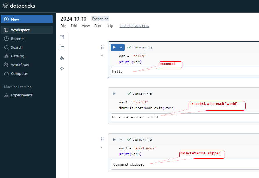
The dbutils.notebook.exit() function is used to terminate the execution of a notebook and return a value to the calling notebook.

After this executed, all below cells commend will skipped, will not execute.

#cell1
var = "hello"
print (var)

#cell2
var2 = "world"
dbutils.notebook.exit(var2)

#cell3
var3 = "good news"
print(var3)

Parent notebook uses child notebook returned value

Parent Notebook
#parent notebook
# Call the child notebook and pass any necessary parameters 
result = dbutils.notebook.run("/Notebooks/child_notebook", 60, {"param1": "some_value"})

#use the child notebook returned value 
print(f"I use the Returned result: {result}")


# Use the result for further logic 
if result == "Success": 
     print("The child notebook completed successfully!") 
else: 
     print("The child notebook encountered an issue.")

child Notebook
#child Notebook
# Simulate some processing (e.g., a query result or a status) 
result_value = "Success" 

# Return the result to the parent notebook 
dbutils.notebook.exit(result_value)

Handling Complex Return Values

Since dbutils.notebook.exit() only returns a string, if you need to return a more complex object (like a dictionary or a list), you need to serialize it to a string format (like JSON) and then deserialize it in the parent notebook.

Child Notebook:

import json

# Simulate a complex return value (a dictionary)
result = {"status": "Success", "rows_processed": 1234}

# Convert the dictionary to a JSON string and exit
dbutils.notebook.exit(json.dumps(result))

Parent Notebook:

import json

# Run the child notebook
result_str = dbutils.notebook.run("/Notebooks/child_notebook", 60, {"param1": "some_value"})

# Convert the returned JSON string back into a dictionary
result = json.loads(result_str)

# Use the values from the result
print(f"Status: {result['status']}")
print(f"Rows Processed: {result['rows_processed']}")

Summary:

  • You can call child notebooks from a parent notebook using Python (dbutils.notebook.run()), but not with SQL directly.
  • You can pass parameters using widgets in the child notebook.
  • Python recommend to use dbutils.get(“parameterName”), still can use getArgument(“parameterName”)
  • SQL use getArgument(“parameterName”) in child notebook only.
  • Results can be returned to the parent notebook using dbutils.notebook.exit().

Please do not hesitate to contact me if you have any questions at William . chen @ mainri.ca

(remove all space from the email account 😊)

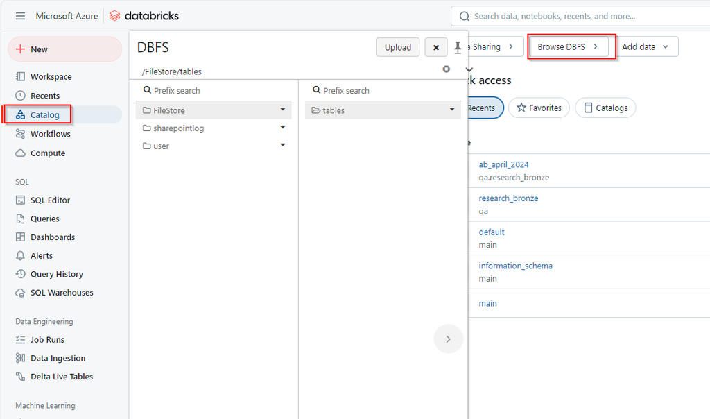
DBFS: Databricks File System (DBFS)

The Databricks File System (DBFS) is a distributed file system integrated with Databricks that allows users to interact with object storage systems like Azure Blob Storage, Amazon S3, and Google Cloud Storage. DBFS enables seamless access to these cloud storage systems within Databricks notebooks and clusters, appearing like a local file system.

Databricks recommends that you store data in mounted object storage rather than in the DBFS root. The DBFS root is not intended for production customer data.

DBFS root is the default file system location provisioned for a Databricks workspace when the workspace is created. It resides in the cloud storage account associated with the Databricks workspace.

Key Features of DBFS

  • Unified Storage Access: DBFS provides a unified interface to interact with various cloud storage platforms (Azure Blob, S3, etc.)
  • Mounting External Storage: DBFS allows you to mount cloud storage containers or buckets so that they are accessible from your Databricks environment like a directory.
  • Persistence: Files written to DBFS in certain directories are persistent and accessible across clusters, ensuring that data is stored and available even when clusters are shut down
  • Interoperability: DBFS integrates with Databricks’ Spark engine, meaning you can read and write data directly into Spark DataFrames,

Structure of DBFS

The Databricks File System is structured similarly to a Unix-like file system. It has the following key components:

  • /FileStore: This is the default directory where you can upload and store small files, such as libraries, scripts, and other assets.
  • /databricks-datasets: This directory contains sample datasets provided by Databricks for learning purposes.
  • /mnt: This is the mount point for external cloud storage, where you can mount and interact with cloud storage services like Azure Blob, AWS S3, or GCS (Google Cloud Storage).

Working with DBFS

List Files in DBFS

dbutils.fs.ls(“/FileStore/”)

Upload Files

dbutils.fs.put(“/FileStore/my_file.txt”, “Hello, DBFS!”, overwrite=True)

Reading Files

df = spark.read.csv(“/FileStore/my_file.csv”, header=True, inferSchema=True)

Writing Files

df.write.csv(“/FileStore/my_output.csv”, mode=”overwrite”)

Mounting External Storage

dbutils.fs.mount(
  source = "wasbs://<container>@<storage-account-name>.blob.core.windows.net",
  mount_point = "/mnt/myblobstorage",
  extra_configs = {"<storage-account-name>.blob.core.windows.net":dbutils.secrets.get(scope = "<scope-name>", key = "<storage-access-key>")})

Unmounting Storage

dbutils.fs.unmount(“/mnt/myblobstorage”)

Conclusion

The Databricks File System (DBFS) is a crucial feature in Databricks that provides seamless, scalable file storage and cloud integration. It abstracts away the complexity of working with distributed storage systems, making it easy to manage and process data. With capabilities like mounting external storage, integration with Spark, and support for various file formats, DBFS is an essential tool for any data engineering or analytics workflow within Databricks.

delta: Schema Evolution

Schema Evolution in Databricks refers to the ability to automatically adapt and manage changes in the structure (schema) of a Delta Lake table over time. It allows users to modify the schema of an existing table (e.g., adding or updating columns) without the need for a complete rewrite of the data.

Key Features of Schema Evolution

  1. Automatic Adaptation: Delta Lake can automatically evolve the schema of a table when new columns are added to the incoming data, or when data types change, if certain configurations are enabled.
  2. Backward and Forward Compatibility: Delta Lake ensures that new data can be written to a table without breaking the existing schema. It also ensures that existing queries remain compatible, even if the schema changes.

Configuration for Schema Evolution

  • mergeSchema
    This option allows you to append new data with a schema that differs from the existing table schema. It merges the new schema into the table.
    Usage: Typically used when you are appending data.
  • overwriteSchema
    This option is used when you want to completely replace the schema of the table with the schema of the new data.
    Usage: Typically used when you are overwriting data

mergSchema

When new data has additional columns that aren’t present in the target Delta table, Delta Lake can automatically merge the new schema into the existing table schema.


# Append new data to the Delta table with automatic schema merging

df_new_data.write.format("delta").mode("append").option("mergeSchema", "true").save("/path/to/delta-table")


overwriteSchema

If you want to replace the entire schema (including removing existing columns), you can use the overwriteSchema option.


# Overwrite the existing Delta table schema with new data

df_new_data.write.format("delta").mode("overwrite").option("overwriteSchema", "true").save("/path/to/delta-table")


Configure spark.databricks.delta.schema.autoMerge

You can configure this setting at the following levels:

  • Session Level (applies to a specific session or job)
  • Cluster Level (applies to all jobs on the cluster)

Session-Level Configuration (Spark session level)

Once this is enabled, all write and merge operations in the session will automatically allow schema evolution.


# Enable auto schema merging for the session

spark.conf.set("spark.databricks.delta.schema.autoMerge.enabled", "true")

Cluster-Level Configuration

This enables automatic schema merging for all operations on the cluster without needing to set it in each job.

  1. Go to your Databricks Workspace.
  2. Navigate to Clusters and select your cluster.
  3. Go to the Configuration tab.
  4. Under Spark Config, add the following configuration:
    spark.databricks.delta.schema.autoMerge.enabled true

Please do not hesitate to contact me if you have any questions at William . chen @ mainri.ca

(remove all space from the email account 😊)

Delta: Time Travel of Delta Table

Time Travel in Delta Lake allows you to query, restore, or audit the historical versions of a Delta table. This feature is useful for various scenarios, including recovering from accidental deletions, debugging, auditing changes, or simply querying past versions of your data.

Delta Lake maintains a transaction log that records all changes (inserts, updates, deletes) made to the table. Using Time Travel, you can access a previous state of the table by specifying a version number or a timestamp.

By default, data file retention is 7 days, log file retention is 30 days. After 7 days, file will delete, but log file still there.

You can access historical versions of a Delta table using two methods:

  1. By Version Number
  2. By Timestamp

Viewing Table History

# sql
DESCRIBE HISTORY my_delta_table;

Query a certain version Table

You can query a Delta table based on a specific version number by using the VERSION AS OF clause. Or timestamp using the TIMESTAMP AS OF clause.


# sql
SELECT * FROM my_delta_table VERSION AS OF 5;


#Python
spark.sql("SELECT * FROM my_delta_table VERSION AS OF 5")

Restore the Delta Table to an Older Version

You can use the RESTORE command to revert the Delta table to a previous state permanently. This modifies the current state of the Delta table to match a past version or timestamp. Delta Lake maintains the transaction log retention period set for the Delta table (by default, 30 days)

#sql
--restore table to earlier version 4
-- by version
RESTORE TABLE delta.`abfss://container@adlsAccount.dfs.windows.net/myDeltaTable` TO VERSION OF 4;

-- by timestamp
RESTORE TABLE my_delta_table TO TIMESTAMP AS OF '2024-10-07T12:30:00';

#python
spark.sql("RESTORE TABLE my_delta_table TO VERSION AS OF 5")
spark.sql("RESTORE TABLE my_delta_table TO TIMESTAMP AS OF '2024-10-07T12:30:00'")

Vacuum Command

The VACUUM command in Delta Lake is used to remove old files that are no longer in use by the Delta table. When you make updates, deletes, or upserts (MERGE) to a Delta table, Delta Lake creates new versions of the data while keeping older versions for Time Travel and data recovery. Over time, these old files can accumulate, consuming storage. The VACUUM command helps clean up these files to reclaim storage space.

This command will remove all files older than 7 days (by Default)


# sql
VACUUM my_delta_table;

# python
spark.sql("VACUUM my_delta_table")

Retention Duration Check

The configuration property


%sql
SET spark.databricks.delta.retentionDurationCheck.enabled = false / true;

spark.databricks.delta.retentionDurationCheck.enable in Delta Lake controls whether Delta Lake enforces the retention period check for the VACUUM operation. By default, Delta Lake ensures that data files are only deleted after the default retention period (typically 7 days) to prevent accidentally deleting files that might still be required for Time Travel or recovery.

When VACUUM is called, Delta Lake checks if the specified retention period is shorter than the minimum default (7 days). If it is, the VACUUM command will fail unless this safety check is disabled.

You can disable this check by setting the property spark.databricks.delta.retentionDurationCheck.enable to false, which allows you to set a retention period of less than 7 days or even vacuum data immediately (0 hours).

Disable the Retention Duration Check


#sql
SET spark.databricks.delta.retentionDurationCheck.enabled = false;

#python
spark.conf.set("spark.databricks.delta.retentionDurationCheck.enabled", "false")

set log Retention Duration


#sql 
# Set the log retention duration to 7 days
SET spark.databricks.delta.logRetentionDuration = '7 days';

# python 
# Set the log retention duration to 7 days
spark.conf.set("spark.databricks.delta.logRetentionDuration", "7 days")


Custom Retention Period


# sql
VACUUM my_delta_table RETAIN 1 HOURS;

# python
spark.sql("VACUUM my_delta_table RETAIN 1 HOURS")

Force Vacuum (Dangerous)


# sql
VACUUM my_delta_table RETAIN 0 HOURS;

Conclusion:

Delta Lake’s Time Travel feature is highly beneficial for data recovery, auditing, and debugging by enabling access to historical data versions. It provides flexibility to query and restore previous versions of the Delta table, helping maintain the integrity of large-scale data operations.

Please do not hesitate to contact me if you have any questions at William . chen @ mainri.ca

(remove all space from the email account 😊)