Comparison of Microsoft Fabric, Azure Synapse Analytics (ASA), Azure Data Factory (ADF), and Azure Databricks (ADB)

Today, data engineers have a wide array of tools and platforms at their disposal for data engineering projects. Popular choices include Microsoft Fabric, Azure Synapse Analytics (ASA), Azure Data Factory (ADF), and Azure Databricks (ADB). It’s common to wonder which one is the best fit for your specific needs.

Side by Side comparison

Here’s a concise comparison of Microsoft Fabric, Azure Synapse Analytics, Azure Data Factory (ADF), and Azure Databricks (ADB) based on their key features, use cases, and differences:

Feature	Microsoft Fabric	Azure Synapse Analytics	Azure Data Factory (ADF)	Azure Databricks (ADB)
Type	Unified SaaS analytics platform	Integrated analytics service	Cloud ETL/ELT service	Apache Spark-based analytics platform
Primary Use Case	End-to-end analytics (Data Engineering, Warehousing, BI, Real-Time)	Large-scale data warehousing & analytics	Data integration & orchestration	Big Data processing, ML, AI, advanced analytics
Data Integration	Built-in Data Factory capabilities	Synapse Pipelines (similar to ADF)	Hybrid ETL/ELT pipelines	Limited (relies on Delta Lake, ADF, or custom code)
Data Warehousing	OneLake (Delta-Parquet based)	Dedicated SQL pools (MPP)	Not applicable	Can integrate with Synapse/Delta Lake
Big Data Processing	Spark-based (Fabric Spark)	Spark pools (serverless/dedicated)	No (orchestration only)	Optimized Spark clusters (Delta Lake)
Real-Time Analytics	Yes (Real-Time Hub)	Yes (Synapse Real-Time Analytics)	No	Yes (Structured Streaming)
Business Intelligence	Power BI (deeply integrated)	Power BI integration	No	Limited (via dashboards or Power BI)
Machine Learning	Basic ML integration	ML in Spark pools	No	Full ML/DL support (MLflow, AutoML)
Pricing Model	Capacity-based (Fabric SKUs)	Pay-as-you-go (serverless) or dedicated	Activity-based	DBU-based (compute + storage)
Open Source Support	Limited (Delta-Parquet)	Limited (Spark, SQL)	No	Full (Spark, Python, R, ML frameworks)
Governance	Centralized (OneLake, Purview)	Workspace-level	Limited	Workspace-level (Unity Catalog)

Key Differences

Fabric vs Synapse: Fabric is a fully managed SaaS (simpler, less configurable), while Synapse offers more control (dedicated SQL pools, Spark clusters).
ADF vs Synapse Pipelines: Synapse Pipelines = ADF inside Synapse (same engine).
ADB vs Fabric Spark: ADB has better ML & open-source support, while Fabric Spark is simpler & integrated with Power BI.

When to Use Which

Microsoft Fabric
- Best for end-to-end analytics in a unified SaaS platform (no infrastructure management).
- Combines data engineering, warehousing, real-time, and BI in one place.
- Good for Power BI-centric organizations.
Azure Synapse Analytics
- Best for large-scale data warehousing with SQL & Spark processing.
- Hybrid of ETL (Synapse Pipelines), SQL Pools, and Spark analytics.
- More flexible than Fabric (supports open formats like Parquet, CSV).
Azure Data Factory (ADF)
- Best for orchestrating ETL/ELT workflows (no compute/storage of its own).
- Used for data movement, transformations, and scheduling.
- Often paired with Synapse or Databricks.
Azure Databricks (ADB)
- Best for advanced analytics, AI/ML, and big data processing with Spark.
- Optimized for Delta Lake (ACID transactions on data lakes).
- Preferred for data science teams needing MLflow, AutoML, etc.

Which One Should You Choose?

For a fully integrated Microsoft-centric solution → Fabric
For large-scale data warehousing + analytics → Synapse
For ETL/data movement → ADF (or Synapse Pipelines)
For advanced Spark-based analytics & ML → Databricks

Data Quality Framework (DQX)

Data quality is more critical than ever in today’s data-driven world. Organizations are generating and collecting vast amounts of data, and the ability to trust and leverage this information is paramount for success. Poor data quality can have severe negative impacts, ranging from flawed decision-making to regulatory non-compliance and significant financial losses.

Key Dimensions of Data Quality (DAMA-DMBOK or ISO 8000 Standards)

A robust DQX evaluates data across multiple dimensions:

Accuracy: Data correctly represents real-world values.
Completeness: No missing or null values where expected.
Consistency: Data is uniform across systems and over time.
Timeliness: Data is up-to-date and available when needed.
Validity: Data conforms to defined business rules (e.g., format, range).
Uniqueness: No unintended duplicates.
Integrity: Relationships between datasets are maintained.

What is Data Quality Framework (DQX)

A Data Quality Framework (DQX) is an open-source framework from Databricks Labs designed to simplify and automate data quality checks for PySpark workloads on both batch and streaming data.

DAX is a structured approach to assessing, monitoring, and improving the quality of data within an organization. It define, validate, and enforce data quality rules across your data pipelines. It ensures that data is accurate, consistent, complete, reliable, and fit for its intended use. so it can be used confidently for analytics, reporting, compliance, and decision-making.

This article will explore how the DQX framework helps improve data reliability, reduce data errors, and enforce compliance with data quality standards. We will step by step go through all steps, from setup and use DQX framework in databricks notebook with code snippets to implement data quality checks.

DQX usage in the Lakehouse Architecture

In the Lakehouse architecture, new data validation should happen during data entry into the curated layer to ensure bad data is not propagated to the subsequent layers. With DQX, you can implement Dead-Letter pattern to quarantine invalid data and re-ingest it after curation to ensure data quality constraints are met. The data quality can be monitored in real-time between layers, and the quarantine process can be automated.

Credits: https://databrickslabs.github.io/dqx/docs/motivation/

Components of a Data Quality Framework

A DQX typically includes:

A. Data Quality Assessment

Profiling: Analyze data to identify anomalies (e.g., outliers, nulls).
Metrics & KPIs: Define measurable standards (e.g., % completeness, error rates).
Benchmarking: Compare against industry standards or past performance.

B. Data Quality Rules & Standards

Define validation rules (e.g., “Email must follow RFC 5322 format”).
Implement checks at the point of entry (e.g., form validation) and during processing.

C. Governance & Roles

Assign data stewards responsible for quality.
Establish accountability (e.g., who fixes issues? Who approves changes?).

D. Monitoring & Improvement

Automated checks: Use tools like Great Expectations, Talend, or custom scripts.
Root Cause Analysis (RCA): Identify why errors occur (e.g., system glitches, human input).
Continuous Improvement: Iterative fixes (e.g., process changes, user training).

E. Tools & Technology

Data Quality Tools: Informatica DQ, IBM InfoSphere, Ataccama, or open-source (Apache Griffin).
Metadata Management: Track data lineage and quality scores.
AI/ML: Anomaly detection (e.g., identifying drift in datasets).

F. Culture & Training

Promote data literacy across teams.
Encourage reporting of data issues without blame.

Using Databricks DQX Framework in a Notebook

Step by Step Implementing DQX

Step 1: Install the DQX Library

install it using the Databricks Labs CLI:

%pip install databricks-labs-dqx

# Restart the kernel after the package is installed in the notebook:
# in a separate cell run:
dbutils.library.restartPython()

Step 2: Initialize the Environment and read input data

Set up the necessary environment for running the Databricks DQX framework, including:

Importing the key components from the Databricks DQX library.

DQProfiler: Used for profiling the input data to understand its structure and generate summary statistics.
DQGenerator: Generates data quality rules based on the profiles.
DQEngine: Executes the defined data quality checks.
WorkspaceClient: Handles communication with the Databricks workspace.

Import Libraries

from databricks.labs.dqx.profiler.profiler import DQProfiler
from databricks.labs.dqx.profiler.generator import DQGenerator
from databricks.labs.dqx.engine import DQEngine
from databricks.sdk import WorkspaceClient

Loading the input data that you want to evaluate.

# Read the input data from a Delta table
input_df = spark.read.table("catalog.schema.table")

Establishing a connection to the Databricks workspace.

# Initialize the WorkspaceClient to interact with the Databricks workspace
ws = WorkspaceClient()

# Initialize a DQProfiler instance with the workspace client
profiler = DQProfiler(ws)

Profiling for data quality.

# Profile the input DataFrame to get summary statistics and data profiles

summary_stats, profiles = profiler.profile(input_df)

Generate DQX quality rules/checks

# generate DQX quality rules/checks
generator = DQGenerator(ws)
checks = generator.generate_dq_rules(profiles)  # with default level "error"

dq_engine = DQEngine(ws)

Save checks in arbitrary workspace location

# save checks in arbitrary workspace location
dq_engine.save_checks_in_workspace_file(checks, workspace_path="/Shared/App1/checks.yml")

Generate DLT expectations

# generate DLT expectations
dlt_generator = DQDltGenerator(ws)

dlt_expectations = dlt_generator.generate_dlt_rules(profiles, language="SQL")
print(dlt_expectations)

dlt_expectations = dlt_generator.generate_dlt_rules(profiles, language="Python")
print(dlt_expectations)

dlt_expectations = dlt_generator.generate_dlt_rules(profiles, language="Python_Dict")
print(dlt_expectations)

The profiler samples 30% of the data (sample ratio = 0.3) and limits the input to 1000 records by default.

Profiling a Table

Tables can be loaded and profiled using profile_table.

from databricks.labs.dqx.profiler.profiler import DQProfiler
from databricks.sdk import WorkspaceClient

# Profile a single table directly
ws = WorkspaceClient()
profiler = DQProfiler(ws)

# Profile a specific table with custom options
summary_stats, profiles = profiler.profile_table(
    table="catalog1.schema1.table1",
    columns=["col1", "col2", "col3"],  # specify columns to profile
    options={
        "sample_fraction": 0.1,  # sample 10% of data
        "limit": 500,            # limit to 500 records
        "remove_outliers": True, # enable outlier detection
        "num_sigmas": 2.5       # use 2.5 standard deviations for outliers
    }
)

print("Summary Statistics:", summary_stats)
print("Generated Profiles:", profiles)

Profiling Multiple Tables

The profiler can discover and profile multiple tables in Unity Catalog. Tables can be passed explicitly as a list or be included/excluded using regex patterns.

from databricks.labs.dqx.profiler.profiler import DQProfiler
from databricks.sdk import WorkspaceClient

ws = WorkspaceClient()
profiler = DQProfiler(ws)

# Profile several tables by name:
results = profiler.profile_tables(
    tables=["main.data.table_001", "main.data.table_002"]
)

# Process results for each table
for summary_stats, profiles in results:
    print(f"Table statistics: {summary_stats}")
    print(f"Generated profiles: {profiles}")

# Include tables matching specific patterns
results = profiler.profile_tables(
    patterns=["$main.*", "$data.*"]
)

# Process results for each table
for summary_stats, profiles in results:
    print(f"Table statistics: {summary_stats}")
    print(f"Generated profiles: {profiles}")

# Exclude tables matching specific patterns
results = profiler.profile_tables(
    patterns=["$sys.*", ".*_tmp"],
    exclude_matched=True
)

# Process results for each table
for summary_stats, profiles in results:
    print(f"Table statistics: {summary_stats}")
    print(f"Generated profiles: {profiles}")

Profiling Options

The profiler supports extensive configuration options to customize the profiling behavior.

from databricks.labs.dqx.profiler.profiler import DQProfiler
from databricks.sdk import WorkspaceClient

# Custom profiling options
custom_options = {
# Sampling options
"sample_fraction": 0.2, # Sample 20% of the data
"sample_seed": 42, # Seed for reproducible sampling
"limit": 2000, # Limit to 2000 records after sampling

# Outlier detection options
"remove_outliers": True, # Enable outlier detection for min/max rules
"outlier_columns": ["price", "age"], # Only detect outliers in specific columns
"num_sigmas": 2.5, # Use 2.5 standard deviations for outlier detection

# Null value handling
"max_null_ratio": 0.05, # Generate is_not_null rule if <5% nulls

# String handling
"trim_strings": True, # Trim whitespace from strings before analysis
"max_empty_ratio": 0.02, # Generate is_not_null_or_empty if <2% empty strings

# Distinct value analysis
"distinct_ratio": 0.01, # Generate is_in rule if <1% distinct values
"max_in_count": 20, # Maximum items in is_in rule list

# Value rounding
"round": True, # Round min/max values for cleaner rules
}

ws = WorkspaceClient()
profiler = DQProfiler(ws)

# Apply custom options to profiling
summary_stats, profiles = profiler.profile(input_df, options=custom_options)

# Apply custom options when profiling tables
tables = [
"dqx.demo.test_table_001",
"dqx.demo.test_table_002",
"dqx.demo.test_table_003", # profiled with default options
]
table_options = {
"dqx.demo.test_table_001": {"limit": 2000},
"dqx.demo.test_table_002": {"limit": 5000},
}
summary_stats, profiles = profiler.profile_tables(tables=tables, options=table_options)

Understanding output

Assuming the sample data is:

customer_id	customer_name	customer_email	is_active	start_date	end_date
1	Alice	alice@mainri.ca	1	2025-01-24	null
2	Bob	bob_new@mainri.ca	1	2025-01-24	null
3	Charlie	invalid_email	1	2025-01-24	null
3	Charlie	invalid_email	0	2025-01-24	2025-01-24

# Initialize the WorkspaceClient to interact with the Databricks workspace
ws = WorkspaceClient()

# Initialize a DQProfiler instance with the workspace client
profiler = DQProfiler(ws)

# Read the input data from a Delta table
input_df = spark.read.table("catalog.schema.table")

# Display a sample of the input data
input_df.display()

# Profile the input DataFrame to get summary statistics and data profiles
summary_stats, profiles = profiler.profile(input_df)

Upon checking the summary and profile of my input data generated, below are the results generated by DQX

print(summary_stats)

Summary of input data on all the columns in input dataframe

# Summary of input data on all the columns in input dataframe
{
  "customer_id": {
    "count": 4,
    "mean": 2.25,
    "stddev": 0.9574271077563381,
    "min": 1,
    "25%": 1,
    "50%": 2,
    "75%": 3,
    "max": 3,
    "count_non_null": 4,
    "count_null": 0
  },
  "customer_name": {
    "count": 4,
    "mean": null,
    "stddev": null,
    "min": "Alice",
    "25%": null,
    "50%": null,
    "75%": null,
    "max": "Charlie",
    "count_non_null": 4,
    "count_null": 0
  },
  "customer_email": {
    "count": 4,
    "mean": null,
    "stddev": null,
    "min": "alice@example.com",
    "25%": null,
    "50%": null,
    "75%": null,
    "max": "charlie@example.com",
    "count_non_null": 4,
    "count_null": 0
  },
  "is_active": {
    "count": 4,
    "mean": 0.75,
    "stddev": 0.5,
    "min": 0,
    "25%": 0,
    "50%": 1,
    "75%": 1,
    "max": 1,
    "count_non_null": 4,
    "count_null": 0
  },
  "start_date": {
    "count": 4,
    "count_non_null": 4,
    "count_null": 0,
    "min": "2025-01-24",
    "max": "2025-01-24",
    "mean": "2025-01-24"
  },
  "end_date": {
    "count": 4,
    "count_non_null": 1,
    "count_null": 3,
    "min": 1737676800,
    "max": 1737676800
  }
}

print(profiles)
# Default Data profile generated based on input data
DQProfile(
  name='is_not_null',
  column='customer_id',
  description=None,
  parameters=None
),
DQProfile(
  name='min_max',
  column='customer_id',
  description='Real min/max values were used',
  parameters={
    'min': 1,
    'max': 3
  }
),
DQProfile(
  name='is_not_null',
  column='customer_name',
  description=None,
  parameters=None
),
DQProfile(
  name='is_not_null',
  column='customer_email',
  description=None,
  parameters=None
),
DQProfile(
  name='is_not_null',
  column='is_active',
  description=None,
  parameters=None
),
DQProfile(
  name='is_not_null',
  column='start_date',
  description=None,
  parameters=None
)

Step 3: Understanding checks applied at data

With the below snippet, we can understand the default checks applied at input data, which generated the data profile as mentioned in previous step.

# generate DQX quality rules/checks
generator = DQGenerator(ws)
checks = generator.generate_dq_rules(profiles)

print(checks)
# Checks applied on input data
[{
  'check': {
    'function': 'is_not_null',
    'arguments': {
      'col_name': 'customer_id'
    }
  },
  'name': 'customer_id_is_null',
  'criticality': 'error'
},
{
  'check': {
    'function': 'is_in_range',
    'arguments': {
      'col_name': 'customer_id',
      'min_limit': 1,
      'max_limit': 3
    }
  },
  'name': 'customer_id_isnt_in_range',
  'criticality': 'error'
},
{
  'check': {
    'function': 'is_not_null',
    'arguments': {
      'col_name': 'customer_name'
    }
  },
  'name': 'customer_name_is_null',
  'criticality': 'error'
},
{
  'check': {
    'function': 'is_not_null',
    'arguments': {
      'col_name': 'customer_email'
    }
  },
  'name': 'customer_email_is_null',
  'criticality': 'error'
},
{
  'check': {
    'function': 'is_not_null',
    'arguments': {
      'col_name': 'is_active'
    }
  },
  'name': 'is_active_is_null',
  'criticality': 'error'
},
{
  'check': {
    'function': 'is_not_null',
    'arguments': {
      'col_name': 'start_date'
    }
  },
  'name': 'start_date_is_null',
  'criticality': 'error'
}]

Step 4: Define custom Data Quality Expectations

In addition to the automatically generated checks, you can define your own custom rules to enforce business-specific data quality requirements. This is particularly useful when your organization has unique validation criteria that aren’t covered by the default checks. By using a configuration-driven approach (e.g., YAML), you can easily maintain and update these rules without modifying your pipeline code.

For example, you might want to enforce that:

Customer IDs must not be null or empty.
Email addresses must match a specific domain format (e.x: @example.com).

# Define custom data quality expectations.
import yaml

checks_custom = yaml.safe_load("""
- check:
    arguments:
        col_name: customer_id
    function: is_not_null_and_not_empty
    criticality: error
    name: customer_id_is_null
- check:
    arguments:
        col_name: customer_email
        regex: '^[A-Za-z0-9._%+-]+@example\.com$'
    function: regex_match
    criticality: error
    name: customer_emaild_is_not_valid""")

# Validate the custom data quality checks
status = DQEngine.validate_checks(checks_custom)

# The above variable for the custom config yaml file can also be pased from workspace file path as given below:
status = DQEngine.validate_checks("path to yaml file in workspace")

# Assert that there are no errors in the validation status
assert not status.has_errors

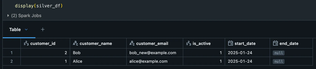
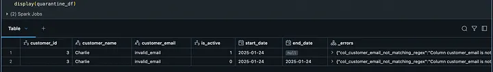
Step 5: Applying the custom rules and generating results

Once your custom data quality rules have been defined and validated, the next step is to apply them to your input data. The DQEngine facilitates this by splitting your dataset into two categories:

Silver Data: Records that meet all quality expectations.
Quarantined Data: Records that fail one or more quality checks.

This approach allows you to separate valid and invalid data for further inspection and remediation. The valid records can proceed to downstream processes, while the quarantined records can be analyzed to determine the cause of failure (e.g., missing values, incorrect formats).

Here’s how you can apply the rules and generate the results:

# Create a DQEngine instance with the WorkspaceClient
dq_engine = DQEngine(WorkspaceClient())

# Apply quality checks and split the DataFrame into silver and quarantine DataFrames
silver_df, quarantine_df = dq_engine.apply_checks_by_metadata_and_split(input_df_1, checks_custom)

Quarantined data – Not matching the rules

Summary

In essence, data quality is no longer just an IT concern; it’s a fundamental business imperative. In today’s complex and competitive landscape, the success of an organization hinges on its ability to leverage high-quality, trusted data for every strategic and operational decision.

A Data Quality Framework (DQX) helps organizations:

Establish clear quality standards
Implement automated checks
Track and resolve issues
Ensure trust in data

https://databrickslabs.github.io/dqx/docs/motivation

https://medium.com/@nivethanvenkat28/revolutionizing-data-quality-checks-using-databricks-dqx-f2a49d83c3c6

Unity Catalog – Table Type Comparison

In Azure Databricks Unity Catalog, you can create different types of tables depending on your storage and management needs. The main table types are including Managed Tables, External Tables, Delta Tables, Foreign Tables, Streaming Tables, Live Tables (deprecated), Feature Tables, and Hive Tables (legacy). Each table type is explained in detail, and a side-by-side comparison is provided for clarity.

Side-by-Side Comparison Table

Feature	Managed Tables	External Tables	Delta Tables	Foreign Tables	Streaming Tables	Delta Live Tables (DLT)	Feature Tables	Hive Tables (Legacy)
Storage	Databricks-managed	External storage	Managed/External	External database	Databricks-managed	Databricks-managed	Managed/External	Managed/External
Location	Internal Delta Lake	Specified external path	Internal/External Delta Lake	External metastore (Snowflake, BigQuery)	Internal Delta Lake	Internal Delta Lake	Internal/External Delta Lake	Internal/External storage
Ownership	Databricks	User	Databricks/User	External provider	Databricks	Databricks	Databricks/User	Databricks (Legacy Hive Metastore)
Deletion Impact	Deletes data & metadata	Deletes only metadata	Depends (Managed: Deletes, External: Keeps data)	Deletes only metadata reference	Deletes data & metadata	Deletes data & metadata	Deletes metadata (but not feature versions)	Similar to Managed/External
Format	Delta Lake	Parquet, CSV, JSON, Delta	Delta Lake	Snowflake, BigQuery, Redshift, etc.	Delta Lake	Delta Lake	Delta Lake	Parquet, ORC, Avro, CSV
Use Case	Full lifecycle management	Sharing with external tools	Advanced data versioning & ACID compliance	Querying external DBs	Continuous data updates	ETL Pipelines	ML feature storage	Legacy storage (pre-Unity Catalog)

Table type and describes

1. Managed Tables

Managed tables are tables where both the metadata and the data are managed by Unity Catalog. When you create a managed table, the data is stored in the default storage location associated with the catalog or schema.

Data Storage and location:

Unity Catalog manages both the metadata and the underlying data in a Databricks-managed location

The data is stored in a Unity Catalog-managed storage location. Typically in an internal Delta Lake storage, e.g., DBFS or Azure Data Lake Storage

Use Case:

Ideal for Databricks-centric workflows where you want Databricks to handle storage and metadata.

Pros & Cons:

Pros: Easy to manage, no need to worry about storage locations.

Cons: Data is tied to Databricks, making it harder to share externally.

Example:

CREATE TABLE managed_table (
    id INT,
    name STRING
);

INSERT INTO managed_table VALUES (1, 'Alice');

SELECT * FROM managed_table;

2. External Tables

External tables store metadata in Unity Catalog but keep data in an external storage location (e.g., Azure Blob Storage, ADLS, S3).

Data storage and Location:

The metadata is managed by Unity Catalog, but the actual data remains in external storage (like Azure Data Lake Storage Gen2 or an S3 bucket).

You must specify an explicit storage location, e.g., Azure Blob Storage, ADLS, S3).

Use Case:

Ideal for cross-platform data sharing or when data is managed outside Databricks.

Pros and Cons

Pros: Data is decoupled from Databricks, making it easier to share.

Cons: Requires manual management of external storage and permissions.

Preparing create external table

Before you can create an external table, you must create a storage credential that allows Unity Catalog to read from and write to the path on your cloud tenant, and an external location that references it.

Requirements

In Azure, create a service principal and grant it the Azure Blob Contributor role on your storage container.
In Azure, create a client secret for your service principal. Make a note of the client secret, the directory ID, and the application ID for the client secret.

step 1: Create a storage credential

You can create a storage credential using the Catalog Explorer or the Unity Catalog CLI. Follow these steps to create a storage credential using Catalog Explorer.

In a new browser tab, log in to Databricks.
Click Catalog.
Click Storage Credentials.
Click Create Credential.
Enter example_credential for he name of the storage credential.
Set Client Secret, Directory ID, and Application ID to the values for your service principal.
Optionally enter a comment for the storage credential.
Click Save.
Leave this browser open for the next steps.

Create an external location

An external location references a storage credential and also contains a storage path on your cloud tenant. The external location allows reading from and writing to only that path and its child directories. You can create an external location from Catalog Explorer, a SQL command, or the Unity Catalog CLI. Follow these steps to create an external location using Catalog Explorer.

Go to the browser tab where you just created a storage credential.
Click Catalog.
Click External Locations.
Click Create location.
Enter example_location for the name of the external location.
Enter the storage container path for the location allows reading from or writing to.
Set Storage Credential to example_credential to the storage credential you just created.
Optionally enter a comment for the external location.
Click Save.

-- Grant access to create tables in the external location
GRANT USE CATALOG
ON example_catalog
TO `all users`;
 
GRANT USE SCHEMA
ON example_catalog.example_schema
TO `all users`;
 
GRANT CREATE EXTERNAL TABLE
ON LOCATION example_location
TO `all users`;

-- Create an example catalog and schema to contain the new table
CREATE CATALOG IF NOT EXISTS example_catalog;
USE CATALOG example_catalog;
CREATE SCHEMA IF NOT EXISTS example_schema;
USE example_schema;

-- Create a new external Unity Catalog table from an existing table
-- Replace <bucket_path> with the storage location where the table will be created
CREATE TABLE IF NOT EXISTS trips_external
LOCATION 'abfss://<bucket_path>'
AS SELECT * from samples.nyctaxi.trips;
 
-- To use a storage credential directly, add 'WITH (CREDENTIAL <credential_name>)' to the SQL statement.

There are some useful Microsoft document to be refer:

“Create an external table in Unity Catalog“
“Configure a managed identity for Unity Catalog“
“Create a Unity Catalog metastore“
“Manage access to external cloud services using service credentials“
“Create a storage credential for connecting to Azure Data Lake Storage Gen2“
“External locations“

Example



CREATE TABLE external_table (
    id INT,
    name STRING
)
LOCATION 'abfss://container@storageaccount.dfs.core.windows.net/path/to/data';

INSERT INTO external_table VALUES (1, 'Bob');

SELECT * FROM external_table;

3. Foreign Tables

Foreign tables reference data stored in external systems (e.g., Snowflake, Redshift) without copying the data into Databricks.

Data Storage and Location

The metadata is stored in Unity Catalog, but the data resides in another metastore (e.g., an external data warehouse like Snowflake or BigQuery).

It does not point to raw files but to an external system.

Use Case:

Best for querying external databases like Snowflake, BigQuery, Redshift without moving data.

Pros and Cons

Pros: No data duplication, seamless integration with external systems.

Cond: Performance depends on the external system’s capabilities.

Example

CREATE FOREIGN TABLE foreign_table
USING com.databricks.spark.snowflake
OPTIONS (
    sfUrl 'snowflake-account-url',
    sfUser 'user',
    sfPassword 'password',
    sfDatabase 'database',
    sfSchema 'schema',
    dbtable 'table'
);

SELECT * FROM foreign_table;

4. Delta Tables

Delta tables use the Delta Lake format, providing ACID transactions, scalable metadata handling, and data versioning.

Data Storage and Location

A special type of managed or external table that uses Delta Lake format.

Can be in managed storage or external storage.

Use Case:

Ideal for reliable, versioned data pipelines.

Pros and Cons

Pros: ACID compliance, time travel, schema enforcement, efficient upserts/deletes.

Cons: Slightly more complex due to Delta Lake features.

Example

CREATE TABLE delta_table (
    id INT,
    name STRING
)
USING DELTA
LOCATION 'abfss://container@storageaccount.dfs.core.windows.net/path/to/delta';

INSERT INTO delta_table VALUES (1, 'Charlie');

SELECT * FROM delta_table;

-- Time travel example
SELECT * FROM delta_table VERSION AS OF 1;

5. Feature Tables

Feature tables are used in machine learning workflows to store and manage feature data for training and inference.

Data Storage and Location

Used for machine learning (ML) feature storage with Databricks Feature Store.

Can be managed or external.

Use Case:

Ideal for managing and sharing features across ML models and teams.

Pros and Cons:

Pros: Centralized feature management, versioning, and lineage tracking.

Example:

from databricks.feature_store import FeatureStoreClient
fs = FeatureStoreClient()
fs.create_table(
    name="feature_table",
    primary_keys=["id"],
    schema="id INT, feature1 FLOAT, feature2 FLOAT",
    description="Example feature table"
)

fs.write_table("feature_table", df, mode="overwrite")
features = fs.read_table("feature_table")

6. Streaming Tables

Streaming tables are designed for real-time data ingestion and processing using Structured Streaming.

Data Location:

Can be stored in managed or external storage.

Use Case:

Ideal for real-time data pipelines and streaming analytics.

Pros and Cons

Pros: Supports real-time data processing, integrates with Delta Lake for reliability.

Cons: Requires understanding of streaming concepts and infrastructure.

Example:

CREATE TABLE streaming_table (
    id INT,
    name STRING
)
USING DELTA;

from pyspark.sql import SparkSession
spark = SparkSession.builder.appName("StreamingExample").getOrCreate()
streaming_df = spark.readStream.format("delta").load("/path/to/delta")
streaming_df.writeStream.format("delta").outputMode("append").start("/path/to/streaming_table")

Delta Live Tables (DLT)

Delta Live Tables (DLT) is the modern replacement for Live Tables. It is a framework for building reliable, maintainable, and scalable ETL pipelines using Delta Lake. DLT automatically handles dependencies, orchestration, and error recovery.

Data storage and Location:

Data is stored in Delta Lake format, either in managed or external storage.

Use Case:

Building production-grade ETL pipelines for batch and streaming data.

DLT pipelines are defined using Python or SQL.
Tables are automatically materialized and can be queried like any other Delta table.

Pros and Cons

Declarative pipeline definition.
Automatic dependency management.
Built-in data quality checks and error handling.
Supports both batch and streaming workloads.

Cons: Requires understanding of Delta Lake and ETL concepts.

Example

import dlt

@dlt.table
def live_table():
    return spark.read.format("delta").load("/path/to/source_table")

8. Hive Tables (Legacy)

Hive tables are legacy tables that use the Apache Hive format. They are supported for backward compatibility.

Data storage Location:

Can be stored in managed or external storage.

Use Case:

Legacy systems or migration projects.

Pros and Cons

Pros: Backward compatibility with older systems.
Cons: Lacks modern features like ACID transactions and time travel.

Example

CREATE TABLE hive_table (
    id INT,
    name STRING
)
STORED AS PARQUET;

INSERT INTO hive_table VALUES (1, 'Dave');
SELECT * FROM hive_table;

Final Thoughts

Use Delta Live Tables for automated ETL pipelines.

Use Feature Tables for machine learning models.

Use Foreign Tables for querying external databases.

Avoid Hive Tables unless working with legacy systems.

Summary

Managed Tables: Fully managed by Databricks, ideal for internal workflows.
External Tables: Metadata managed by Databricks, data stored externally, ideal for cross-platform sharing.
Delta Tables: Advanced features like ACID transactions and time travel, ideal for reliable pipelines.
Foreign Tables: Query external systems without data duplication.
Streaming Tables: Designed for real-time data processing.
Feature Tables: Specialized for machine learning feature management.
Hive Tables: Legacy format, not recommended for new projects.

Each table type has its own creation syntax and usage patterns, and the choice depends on your specific use case, data storage requirements, and workflow complexity.

Please do not hesitate to contact me if you have any questions at William . chen @ mainri.ca

(remove all space from the email account 😊)

Implementing Slowly Changing Dimension Type 2 Using Delta Lake on Databricks

Built on Apache Spark, Delta Lake provides a robust storage layer for data in Delta tables. Its features include ACID transactions, high-performance queries, schema evolution, and data versioning, among others.

Today’s focus is on how Delta Lake simplifies the management of slowly changing dimensions (SCDs).

Quickly review Type 2 of Slowly Changing Dimension

A quick recap of SCD Type 2 follows:

Storing historical dimension data with effective dates.
Keeping a full history of dimension changes (with start/end dates).
Adding new rows for dimension changes (preserving history).

# Existing Dimension data
surrokey  depID   dep	StartDate   EndDate     IsActivity
1	  1001	  IT	2019-01-01  9999-12-31  1
2	  1002	  Sales	2019-01-01  9999-12-31  1
3	  1003	  HR	2019-01-01  9999-12-31  1

# Dimension changed and new data comes 
depId dep
1003  wholesale   <--- depID is same, name changed from "Sales" to "wholesale"
1004  Finance     <--- new data

# the new Dimension will be:
surrokey  depID	dep	   StartDate   EndDate     IsActivity 
1	  1001	IT	   2019-01-01  9999-12-31  1   <-- No action required
2	  1002	HR	   2019-01-01  9999-12-31  1   <-- No action required
3	  1003	Sales	   2019-01-01  2020-12-31  0   <-- mark as inactive
4         1003  wholesale  2021-01-01  9999-12-31  1   <-- add updated active value
5         1004  Finance    2021-01-01  9999-12-31  1   <-- insert new data

Creating demo data

We’re creating a Delta table, dim_dep, and inserting three rows of existing dimension data.

Existing dimension data

%sql
# Create table dim_dep
%sql
create table dim_dep (
Surrokey BIGINT  GENERATED ALWAYS AS IDENTITY
, depID  int
, dep	string
, StartDate   DATE 
, End_date DATE 
, IsActivity BOOLEAN
)
using delta
location 'dbfs:/mnt/dim/'

# Insert data
insert into dim_dep (depID,dep, StartDate,EndDate,IsActivity) values
(1001,'IT','2019-01-01', '9999-12-31' , 1),
(1002,'Sales','2019-01-01', '9999-12-31' , 1),
(1003,'HR','2019-01-01', '9999-12-31' , 1)

select * from dim_dep
Surrokey depID	dep	StartDate	EndDate	        IsActivity
1	 1001	IT	2019-01-01	9999-12-31	true
2	 1002	Sales	2019-01-01	9999-12-31	true
3	 1003	HR	2019-01-01	9999-12-31	true

%python
dbutils.fs.ls('dbfs:/mnt/dim')
path	name	size	modificationTime
Out[43]: [FileInfo(path='dbfs:/mnt/dim/_delta_log/', name='_delta_log/', size=0, modificationTime=0),
 FileInfo(path='dbfs:/mnt/dim/part-00000-5f9085db-92cc-4e2b-886d-465924de961b-c000.snappy.parquet', name='part-00000-5f9085db-92cc-4e2b-886d-465924de961b-c000.snappy.parquet', size=1858, modificationTime=1736027755000)]

New coming source data

The new coming source data which may contain new record or updated record.

Dimension changed and new data comes 
depId       dep
1002        wholesale 
1003        HR  
1004        Finance

depID 1002, dep changed from “Sales” to “wholesale”, updating dim_dep table;
depID 1003, nothing changed, no action required
depID 1004, is a new record, inserting into dim_dep

Assuming the data, originating from other business processes, is now stored in the data lake as CSV files.

Implementing SCD Type 2

Step 1: Read the source

%python 
df_dim_dep_source = spark.read.csv('dbfs:/FileStore/dep.csv', header=True)

df_dim_dep_source.show()
+-----+---------+
|depid|      dep|
+-----+---------+
| 1002|Wholesale|
| 1003|       HR|
| 1004|  Finance|
+-----+---------+

Step 2: Read the target

df_dim_dep_target = spark.read.format("delta").load("dbfs:/mnt/dim/")

df_dim_dep_target.show()
+--------+-----+-----+----------+----------+----------+
|Surrokey|depID|  dep| StartDate|   EndDate|IsActivity|
+--------+-----+-----+----------+----------+----------+
|       1| 1001|   IT|2019-01-01|9999-12-31|      true|
|       2| 1002|Sales|2019-01-01|9999-12-31|      true|
|       3| 1003|   HR|2019-01-01|9999-12-31|      true|
+--------+-----+-----+----------+----------+----------+

Step 3: Source Left outer Join Target

We perform a source dataframe – df_dim_dep_source, left outer join target dataframe – df_dim_dep_target, where source depID = target depID, and also target’s IsActivity = 1 (meant activity)

This join’s intent is not to miss any new data coming through source. And active records in target because only for those data SCD update is required. After joining source and target, the resultant dataframe can be seen below.

src = df_dim_dep_source
tar = df_dim_dep_target
df_joined = src.join (tar,\
        (src.depid == tar.depID) \
         & (tar.IsActivity == 'true')\
        ,'left') \
    .select(src['*'] \
        , tar.Surrokey.alias('tar_surrokey')\
        , tar.depID.alias('tar_depID')\
        , tar.dep.alias('tar_dep')\
        , tar.StartDate.alias('tar_StartDate')\
        , tar.EndDate.alias('tar_EndDate')\
        , tar.IsActivity.alias('tar_IsActivity')   )
    
df_joined.show()
+-----+---------+------------+---------+-------+-------------+-----------+--------------+
|depid|      dep|tar_surrokey|tar_depID|tar_dep|tar_StartDate|tar_EndDate|tar_IsActivity|
+-----+---------+------------+---------+-------+-------------+-----------+--------------+
| 1002|Wholesale|           2|     1002|  Sales|   2019-01-01| 9999-12-31|          true|
| 1003|       HR|           3|     1003|     HR|   2019-01-01| 9999-12-31|          true|
| 1004|  Finance|        null|     null|   null|         null|       null|          null|
+-----+---------+------------+---------+-------+-------------+-----------+--------------+

Step 4: Filter only the non matched and updated records

In this demo, we only have depid and dep two columns. But in the actual development environment, may have many many columns.

Instead of comparing multiple columns, e.g.,
src_col1 != tar_col1,
src_col2 != tar_col2,
…..
src_colN != tar_colN
We compute hashes for both column combinations and compare the hashes. In addition of this, in case of column’s data type is different, we convert data type the same one.

from pyspark.sql.functions import col , xxhash64

df_filtered = df_joined.filter(\
    xxhash64(col('depid').cast('string'),col('dep').cast('string')) \
    != \
    xxhash64(col('tar_depID').cast('string'),col('tar_dep').cast('string'))\
    )
    
df_filtered.show()
+-----+---------+------------+---------+-------+-------------+-----------+--------------+
|depid|      dep|tar_surrokey|tar_depID|tar_dep|tar_StartDate|tar_EndDate|tar_IsActivity|
+-----+---------+------------+---------+-------+-------------+-----------+--------------+
| 1002|Wholesale|           2|     1002|  Sales|   2019-01-01| 9999-12-31|          true|
| 1004|  Finance|        null|     null|   null|         null|       null|          null|
+-----+---------+------------+---------+-------+-------------+-----------+--------------+

from the result, we can see:

The row, dep_id = 1003, dep = HR, was filtered out because both source and target side are the same. No action required.
The row, depid =1002, dep changed from “Sales” to “Wholesale”, need updating.
The row, depid = 1004, Finance is brand new row, need insert into target side – dimension table.

Step 5: Find out records that will be used for inserting

From above discussion, we have known depid=1002, need updating and depid=1004 is a new rocord. We will create a new column ‘merge_key’ which will be used for upsert operation. This column will hold the values of source id.

Add a new column – “merge_key”

df_inserting = df_filtered. withColumn('merge_key', col('depid'))

df_inserting.show()
+-----+---------+------------+---------+-------+-------------+-----------+--------------+---------+
|depid|      dep|tar_surrokey|tar_depID|tar_dep|tar_StartDate|tar_EndDate|tar_IsActivity|merge_key|
+-----+---------+------------+---------+-------+-------------+-----------+--------------+---------+
| 1002|Wholesale|           2|     1002|  Sales|   2019-01-01| 9999-12-31|          true|     1002|
| 1004|  Finance|        null|     null|   null|         null|       null|          null|     1004|
+-----+---------+------------+---------+-------+-------------+-----------+--------------+---------+
The above 2 records will be inserted as new records to the target table

The above 2 records will be inserted as new records to the target table.

Step 6: Find out the records that will be used for updating in target table

from pyspark.sql.functions import lit
df_updating = df_filtered.filter(col('tar_depID').isNotNull()).withColumn('merge_key',lit('None')

df_updating.show()
+-----+---------+------------+---------+-------------+-----------+--------------+---------+
|depid|      dep|tar_surrokey|tar_depID|tar_StartDate|tar_EndDate|tar_IsActivity|merge_key|
+-----+---------+------------+---------+-------------+-----------+--------------+---------+
| 1003|Wholesale|           3|     1003|   2019-01-01| 9999-12-31|          true|     None|
+-----+---------+------------+---------+-------------+-----------+--------------+---------+
The above record will be used for updating SCD columns in the target table.

This dataframe filters the records that have tar_depID column not null which means, the record already exists in the table for which SCD update has to be done. The column merge_key will be ‘None’ here which denotes this only requires update in SCD cols.

Step 7: Combine inserting and updating records as stage

df_stage_final = df_updating.union(df_instering)

df_stage_final.show()
+-----+---------+------------+---------+-------+-------------+-----------+--------------+---------+
|depid|      dep|tar_surrokey|tar_depID|tar_dep|tar_StartDate|tar_EndDate|tar_IsActivity|merge_key|
+-----+---------+------------+---------+-------+-------------+-----------+--------------+---------+
| 1002|Wholesale|           2|     1002|  Sales|   2019-01-01| 9999-12-31|          true|     None| <-- updating in SCD table
| 1002|Wholesale|           2|     1002|  Sales|   2019-01-01| 9999-12-31|          true|     1002| <-- inserting in SCD table
| 1004|  Finance|        null|     null|   null|         null|       null|          null|     1004| <-- inserting in SCD table
+-----+---------+------------+---------+-------+-------------+-----------+--------------+---------+

records with merge_key as none are for updating in existing dimension table.
records with merge_key not null will be inserted as new records in dimension table.

Step 8: Upserting the dim_dep Dimension Table

Before performing the upsert, let’s quickly review the existing dim_dep table and the incoming source data.

# Existing dim_dep table
spark.read.table('dim_dep').show()
+--------+-----+-----+----------+----------+----------+
|Surrokey|depID|  dep| StartDate|   EndDate|IsActivity|
+--------+-----+-----+----------+----------+----------+
|       1| 1001|   IT|2019-01-01|9999-12-31|      true|
|       2| 1002|Sales|2019-01-01|9999-12-31|      true|
|       3| 1003|   HR|2019-01-01|9999-12-31|      true|
+--------+-----+-----+----------+----------+----------+

# coming updated source data
park.read.csv('dbfs:/FileStore/dep_src.csv', header=True).show()
+-----+---------+
|depid|      dep|
+-----+---------+
| 1002|Wholesale|
| 1003|       HR|
| 1004|  Finance|
+-----+---------+

Implementing an SCD Type 2 UpSert on the dim_dep Dimension Table

from delta.tables import DeltaTable
from pyspark.sql.functions import current_date, to_date, lit

# define the source DataFrame
src = df_stage_final  # this is a DataFrame object

# Load the target Delta table
tar = DeltaTable.forPath(spark, "dbfs:/mnt/dim")  # target Dimension table


# Performing the UpSert
tar.alias("tar").merge(
    src.alias("src"),
    condition="tar.depID == src.merge_key and tar_IsActivity = 'true'"
).whenMatchedUpdate( \
    set = { \
        "IsActivity": "'false'", \
        "EndDate": "current_date()" \
        }) \
.whenNotMatchedInsert( \
    values = \
    {"depID": "src.depid", \
    "dep": "src.dep", \
    "StartDate": "current_date ()", \
    "EndDate": """to_date('9999-12-31', 'yyyy-MM-dd')""", \
    "IsActivity": "'true' \
    "}) \
.execute()

all done!

Validating the result

spark.read.table('dim_dep').sort(['depID','Surrokey']).show()
+--------+-----+---------+----------+----------+----------+
|Surrokey|depID|      dep| StartDate|   EndDate|IsActivity|
+--------+-----+---------+----------+----------+----------+
|       1| 1001|       IT|2019-01-01|9999-12-31|      true|
|       2| 1002|    Sales|2019-01-01|2020-01-05|     false| <--inactived
|       4| 1002|Wholesale|2020-01-05|9999-12-31|      true| <--updated status
|       3| 1003|       HR|2019-01-01|9999-12-31|      true|
|       5| 1004|  Finance|2020-01-05|9999-12-31|      true| <--append new record
+--------+-----+---------+----------+----------+----------+

Conclusion

we demonstrated how to unlock the power of Slowly Changing Dimension (SCD) Type 2 using Delta Lake, a revolutionary storage layer that transforms data lakes into reliable, high-performance, and scalable repositories. With this approach, organizations can finally unlock the full potential of their data and make informed decisions with confidence

Please do not hesitate to contact me if you have any questions at William . chen @ mainri.ca

(remove all space from the email account 😊)

PySpark Data sources

PySpark supports a variety of data sources, enabling seamless integration and processing of structured and semi-structured data from multiple formats. such as CSV, JSON, Parquet, and ORC, Database (JDBC), as well as more advanced formats like Avro and Delta Lake, Hive

Query Database Table

df = spark.read \
    .format("jdbc") \
    .option("url", "jdbc:mysql://{server_name}:{port}/{database_name}") \
    .option("driver", "com.mysql.cj.jdbc.Driver") \
    .option("dbtable", "employee") \
    .option("user", "root") \
    .option("password", "root") \
    .load()

# Query table using jdbc()
# Parameters
server_name = "myserver.database.windows.net"
port = "1433"
database_name = "mydatabase"
table_name = "mytable"
username = "myusername"
password = "mypassword"

# Construct the JDBC URL
jdbc_url = f"jdbc:sqlserver://{server_name}:{port};databaseName={database_name}"
connection_properties = {
    "user": username,
    "password": password,
    "driver": "com.microsoft.sqlserver.jdbc.SQLServerDriver"
}

# Read data from the SQL database
df = spark.read.jdbc(url=jdbc_url, table=table_name, properties=connection_properties)
# show DataFrame
df_dep.show()
+-----+--------------+
|depid|           dep|
+-----+--------------+
|    1|            IT|
|    2|          Sale|
|    3|       Finance|
|    4|human resource|
+-----+--------------+

Query JDBC Table Parallel, specific Columns

df = spark.read \
    .format("jdbc") \
    .option("url", "jdbc:mysql://localhost:3306/emp") \
    .option("driver", "com.mysql.cj.jdbc.Driver") \
    .option("query", "select id,age from emp where sex='M'") \
    .option("numPartitions",5) \
    .option("fetchsize", 20) \
    .option("user", "root") \
    .option("password", "root") \
    .load()

df.show()

Read & Write CSV File

Read CSV File

df = spark.read.format("csv")\
.options(delimiter=',') \
.options(inferSchema='True')\
.options(header='True')\
.load("/Folder/, /filePath2/")

Write CSV File

df = spark.write.format("csv")\
.options(delimiter=',') \
.options(inferSchema='True')\
.options(header='True')\
.mode("overwrite")
.save("/filePath/filename")

By default, If you try to write directly to a file (e.g., name1.csv), it conflicts because Spark doesn’t generate a single file but a collection of part files in a directory.

path
dbfs:/FileStore/name1.csv/_SUCCESS
dbfs:/FileStore/name1.csv/_committed_7114979947112568022
dbfs:/FileStore/name1.csv/_started_7114979947112568022
dbfs:/FileStore/name1.csv/part-00000-tid-7114979947112568022-b2482528-b2f8-4c82-82fb-7c763d91300e-12-1-c000.csv

PySpark writes data in parallel, which results in multiple part files rather than a single CSV file by default. However, you can consolidate the data into a single CSV file by performing a coalesce(1) or repartition(1) operation before writing, which reduces the number of partitions to one.

df.coalesce(1).write.format("csv").mode("overwrite").options(header=True).save("dbfs:/FileStore/name1.csv")

at this time, name1.csv in “dbfs:/FileStore/name1.csv” will treat as a directory, rather than a Filename. PySpark writes the single file with a random name like part-00000-<id>.csv

dbfs:/FileStore/name1.csv/part-00000-tid-4656450869948503591-85145263-6f01-4b56-ad37-3455ca9a8882-9-1-c000.csv

we need take additional step – “Rename the File to name1.csv“

# List all files in the directory
files = dbutils.fs.ls("dbfs:/FileStore/name1.csv")

# Filter for the part file
for file in files:
    if file.name.startswith("part-"):
        source_file = file.path  # Full path to the part file
        destination_file = "dbfs:/FileStore/name1.csv"
        
        # Move and rename the file
        dbutils.fs.mv(source_file, destination_file)
        break


display(dbutils.fs.ls ( "dbfs:/FileStore/"))

Direct Write with Custom File Name

PySpark doesn’t natively allow specifying a custom file name directly while writing a file because it writes data in parallel using multiple partitions. However, you can achieve a custom file name with a workaround. Here’s how:

Steps:

Use coalesce(1) to combine all data into a single partition.
Save the file to a temporary location.
Rename the part file to the desired name.

# Combine all data into one partition
df.coalesce(1).write.format("csv") \
    .option("header", "true") \
    .mode("overwrite") \
    .save("dbfs:/FileStore/temp_folder")

# Get the name of the part file
files = dbutils.fs.ls("dbfs:/FileStore/temp_folder")
for file in files:
    if file.name.startswith("part-"):
        part_file = file.path
        break

# Move and rename the part file
dbutils.fs.mv(part_file, "dbfs:/FileStore/name1.csv")

# Remove the temporary folder
dbutils.fs.rm("dbfs:/FileStore/temp_folder", True)

Read & Write Parquet File

sample data save at /tmp/output/people.parquet

dbfs:/tmp/output/people.parquet/part-00007-tid-4023475225384587157-553904a7-7460-4fb2-a4b8-140ccc85024c-15-1-c000.snappy.parquet

read from parquet

sample data save at /tmp/output/people.parquet
df1=spark.read.parquet("/tmp/output/people.parquet")
+---------+----------+--------+-----+------+------+
|firstname|middlename|lastname|  dob|gender|salary|
+---------+----------+--------+-----+------+------+
|   James |          |   Smith|36636|     M|  3000|
| Michael |      Rose|        |40288|     M|  4000|
|  Robert |          |Williams|42114|     M|  4000|
|   Maria |      Anne|   Jones|39192|     F|  4000|
|      Jen|      Mary|   Brown|     |     F|    -1|
+---------+----------+--------+-----+------+------+

read a parquet is the same as reading from csv, nothing special.

write to a parquet

append: appends the data from the DataFrame to the existing file, if the Destination files already exist. In Case the Destination files do not exists, it will create a new parquet file in the specified location.

df.write.mode(“append”).parquet(“path/to/parquet/file”)
overwrite: This mode overwrites the destination Parquet file with the data from the DataFrame. If the file does not exist, it creates a new Parquet file.

df.write.mode(“overwrite”).parquet(“path/to/parquet/file”)
ignore: If the destination Parquet file already exists, this mode does nothing and does not write the DataFrame to the file. If the file does not exist, it creates a new Parquet file.

df.write.mode(“ignore”).parquet(“path/to/parquet/file”)
Create Parquet partition file

df.write.partitionBy(“gender”,”salary”).mode(“overwrite”).parquet(“/tmp/output/people2.parquet”)

Read & write Delta Table in PySpark

Read from a Delta Table

Read from a Registered Delta Table (in the Catalog)

df = spark.read.table("default.dim_dep")

df.show()
+--------+-----+-----+----------+----------+----------+
|Surrokey|depID|  dep| StartDate|   EndDate|IsActivity|
+--------+-----+-----+----------+----------+----------+
|       1| 1001|   IT|2019-01-01|9999-12-31|      true|
|       2| 1002|Sales|2019-01-01|9999-12-31|      true|
|       3| 1003|   HR|2019-01-01|9999-12-31|      true|
+--------+-----+-----+----------+----------+----------+

Read from a Delta Table Stored in a Directory (Path-Based)

df_delta_table = spark.read.format("delta").load("dbfs:/mnt/dim/")

df_delta_table.show()
+--------+-----+-----+----------+----------+----------+
|Surrokey|depID|  dep| StartDate|   EndDate|IsActivity|
+--------+-----+-----+----------+----------+----------+
|       1| 1001|   IT|2019-01-01|9999-12-31|      true|
|       2| 1002|Sales|2019-01-01|9999-12-31|      true|
|       3| 1003|   HR|2019-01-01|9999-12-31|      true|
+--------+-----+-----+----------+----------+----------+

Write to a Delta Table

Append to a Delta Table

# Appends to the Delta table
df.write.format("delta").mode("append").save("dbfs:/mnt/dim/")

Overwrite a Delta Table

# Overwrites the Delta table
df.write.format("delta").mode("overwrite").save("dbfs:/mnt/dim/")

Create or Overwrite a Registered Delta Table

# Overwrites the table in the catalog
df.write.format("delta").mode("overwrite").saveAsTable("default.dim_dep")

Append to a Registered Delta Table:

# Appends to the table in the catalog
df.write.format("delta").mode("append").saveAsTable("default.dim_dep")

merge operation (upsert)

from delta.tables import DeltaTable
from pyspark.sql.functions import current_date, lit

# Perform the merge operation
target_table.alias("t").merge(
    source_df.alias("s"),
    "t.id = s.id"  # Join condition: match rows based on `id`
).whenMatchedUpdate(
    set={
        "name": "s.name",  # Update `name` column
        "date": "s.date"   # Update `date` column
    }
).whenNotMatchedInsert(
    values={
        "id": "s.id",      # Insert `id`
        "name": "s.name",  # Insert `name`
        "date": "s.date"   # Insert `date`
    }
).execute()

# Verify the result
result_df = spark.read.format("delta").load(target_table_path)
result_df.show()

Explanation of the Code

Target Table (target_table):
- The Delta table is loaded using DeltaTable.forPath.
- This table contains existing data where updates or inserts will be applied.
Source DataFrame (source_df):
- This DataFrame contains new or updated records.
Join Condition ("t.id = s.id"):
- Rows in the target table (t) are matched with rows in the source DataFrame (s) based on id.
whenMatchedUpdate:
- If a matching row is found, update the name and date columns in the target table.
whenNotMatchedInsert:
- If no matching row is found, insert the new record from the source DataFrame into the target table.
execute():
- Executes the merge operation, applying updates and inserts.
Result Verification:
- After the merge, the updated Delta table is read and displayed.

Schema Evolution

df.write.format("delta").option("mergeSchema", "true").mode("append").save("dbfs:/mnt/dim/")

Read & Write JSON file

Read a simple JSON file

# Read a simple JSON file into dataframe
{
  "RecordNumber": 10,
  "Zipcode": 709,
  "ZipCodeType": "STANDARD",
  "City": "BDA SAN LUIS",
  "State": "PR"
}

df_simple = spark.read.format("json") \
.option("multiline","True")\
.load("dbfs:/FileStore/simple_json.json")

df_simple.printSchema()
root
 |-- City: string (nullable = true)
 |-- RecordNumber: long (nullable = true)
 |-- State: string (nullable = true)
 |-- ZipCodeType: string (nullable = true)
 |-- Zipcode: long (nullable = true)

df_simple.show()
+------------+------------+-----+-----------+-------+
|        City|RecordNumber|State|ZipCodeType|Zipcode|
+------------+------------+-----+-----------+-------+
|BDA SAN LUIS|          10|   PR|   STANDARD|    709|
+------------+------------+-----+-----------+-------+

pay attention on “.option(“multiline”,”True”)“. since my json file is multiple lines (look at above sample data), if reading without this option, it can still run load. But the dataframe will not work. Once you show, you will get this error

df_simple = spark.read.format(“json”).load(“dbfs:/FileStore/simple_json.json”)
df_simple,show()

AnalysisException: Since Spark 2.3, the queries from raw JSON/CSV files are disallowed when the referenced columns only include the internal corrupt record column (named _corrupt_record by default).

Reading from Multiline JSON (JSON Array) File

[{
  "RecordNumber": 2,
  "Zipcode": 704,
  "ZipCodeType": "STANDARD",
  "City": "PASEO COSTA DEL SUR",
  "State": "PR"
},
{
  "RecordNumber": 10,
  "Zipcode": 709,
  "ZipCodeType": "STANDARD",
  "City": "BDA SAN LUIS",
  "State": "PR"
}]
df_jsonarray_simple = spark.read\
    .format("json")\
    .option("multiline", "true")\
    .load("dbfs:/FileStore/jsonArrary.json")

df_jsonarray_simple.show()
+-------------------+------------+-----+-----------+-------+
|               City|RecordNumber|State|ZipCodeType|Zipcode|
+-------------------+------------+-----+-----------+-------+
|PASEO COSTA DEL SUR|           2|   PR|   STANDARD|    704|
|       BDA SAN LUIS|          10|   PR|   STANDARD|    709|
+-------------------+------------+-----+-----------+-------+

read complex json

df_complexjson=spark.read\
    .option("multiline","true")\
    .json("dbfs:/FileStore/jsonArrary2.json")

df_complexjson.select("id","type","name","ppu","batters","topping").show(truncate=False, vertical=True)
-RECORD 0--------------------------------------------------------------------------------------------------------------------------------------------
 id      | 0001                                                                                                                                      
 type    | donut                                                                                                                                     
 name    | Cake                                                                                                                                      
 ppu     | 0.55                                                                                                                                      
 batters | {[{1001, Regular}, {1002, Chocolate}, {1003, Blueberry}, {1004, Devil's Food}]}                                                           
 topping | [{5001, None}, {5002, Glazed}, {5005, Sugar}, {5007, Powdered Sugar}, {5006, Chocolate with Sprinkles}, {5003, Chocolate}, {5004, Maple}] 
-RECORD 1--------------------------------------------------------------------------------------------------------------------------------------------
 id      | 0002                                                                                                                                      
 type    | donut                                                                                                                                     
 name    | Raised                                                                                                                                    
 ppu     | 0.55                                                                                                                                      
 batters | {[{1001, Regular}]}                                                                                                                       
 topping | [{5001, None}, {5002, Glazed}, {5005, Sugar}, {5003, Chocolate}, {5004, Maple}]                                                           
-RECORD 2--------------------------------------------------------------------------------------------------------------------------------------------
 id      | 0003                                                                                                                                      
 type    | donut                                                                                                                                     
 name    | Old Fashioned                                                                                                                             
 ppu     | 0.55                                                                                                                                      
 batters | {[{1001, Regular}, {1002, Chocolate}]}                                                                                                    
 topping | [{5001, None}, {5002, Glazed}, {5003, Chocolate}, {5004, Maple}]

Reading from Multiple files at a time

# Read multiple files
df2 = spark.read.json(
    ['resources/zipcode1.json','resources/zipcode2.json'])

Reading from Multiple files at a time

# Read all JSON files from a folder
df3 = spark.read.json("resources/*.json")

Reading files with a user-specified custom schema

# Define custom schema
schema = StructType([
      StructField("RecordNumber",IntegerType(),True),
      StructField("Zipcode",IntegerType(),True),
      StructField("ZipCodeType",StringType(),True),
      StructField("City",StringType(),True),
      StructField("State",StringType(),True),
      StructField("LocationType",StringType(),True),
      StructField("Lat",DoubleType(),True),
      StructField("Long",DoubleType(),True),
      StructField("Xaxis",IntegerType(),True),
      StructField("Yaxis",DoubleType(),True),
      StructField("Zaxis",DoubleType(),True),
      StructField("WorldRegion",StringType(),True),
      StructField("Country",StringType(),True),
      StructField("LocationText",StringType(),True),
      StructField("Location",StringType(),True),
      StructField("Decommisioned",BooleanType(),True),
      StructField("TaxReturnsFiled",StringType(),True),
      StructField("EstimatedPopulation",IntegerType(),True),
      StructField("TotalWages",IntegerType(),True),
      StructField("Notes",StringType(),True)
  ])

df_with_schema = spark.read.schema(schema) \
        .json("resources/zipcodes.json")
df_with_schema.printSchema()

Reading File using PySpark SQL

spark.sql("CREATE OR REPLACE TEMPORARY VIEW zipcode USING json OPTIONS" + 
      " (path 'resources/zipcodes.json')")
spark.sql("select * from zipcode").show()

Write to JSON

Options

path: Specifies the path where the JSON files will be saved.
mode: Specifies the behavior when writing to an existing directory.
compression: Specifies the compression codec to use when writing the JSON files (e.g., “gzip”, “snappy”).
df2.write . option(“compression”, “gzip”)
dateFormat: Specifies the format for date and timestamp columns.
df.write . option(“dateFormat”, “yyyy-MM-dd”)
timestampFormat: Specifies the format for timestamp columns.
df.write . option(“timestampFormat“, “yyyy-MM-dd’T’HH:mm:ss.SSSXXX”)
lineSep: Specifies the character sequence to use as a line separator between JSON objects. \n (Unix/Linux newline); \r\n (Windows newline)
df . write . option(“lineSep”, “\r\n”)
encoding: Specifies the character encoding to use when writing the JSON files.
UTF-8, UTF-16, ISO-8859-1 (Latin-1), Other Java-supported encodings.
df . write . option(“encoding”, “UTF-8”)

df2.write . format("json")
 . option("compression", "gzip") \
 . option("dateFormat", "yyyy-MM-dd") \ 
 . option("timestampFormat", "yyyy-MM-dd'T'HH:mm:ss.SSSXXX") \
 . option("encoding", "UTF-8") \
 . option("lineSep", "\r\n")
 . save("dbfs:/FileStore/output_json")

modes

Append: Appends the data to the existing data in the target location. If the target location does not exist, it creates a new one.
Overwrite: Overwrites the data in the target location if it already exists. If the target location does not exist, it creates a new one.
Ignore: Ignores the operation and does nothing if the target location already exists. If the target location does not exist, it creates a new one.
Error or ErrorIfExists: Throws an error and fails the operation if the target location already exists. This is the default behavior if no saving mode is specified.

# Write with savemode example
df2.write.mode('Overwrite').json("/tmp/spark_output/zipcodes.json")

Read & Write SQL Server

Read from SQL Server

server_name = "mainri-sqldb.database.windows.net"
port=1433
username="my login name"
password="my login password"
database_name="mainri-sqldb"
table_name="dep"

jdbc_url = f"jdbc:sqlserver://{server_name}:{port};databaseName={database_name}"
connection_properties = {
    "user": username,
    "password": password,
    "driver": "com.microsoft.sqlserver.jdbc.SQLServerDriver"
}
df = spark.read.jdbc(url=jdbc_url, table=table_name, properties=connection_properties)
df.show()
+-----+--------------+
|depid|           dep|
+-----+--------------+
|    1|            IT|
|    2|          Sale|
|    3|       Finance|
|    4|human resource|
+-----+--------------+

alternative way

df1=spark.read \
  .format("jdbc") \
  .option("url", jdbc_url) \
  .option("dbtable", table_name) \
  .option("user", username) \
  .option("password", password) \
  .load()

Select Specific Columns to Read

In the above example, it reads the entire table into PySpark DataFrame. Sometimes you may not be required to select the entire table, so to select the specific columns, specify the query you wanted to select with dbtable option.

df1=spark.read \
  .format("jdbc") \
  .option("url", jdbc_url) \
  .option("databaseName",database_name) \
  .option("query", "select * from [dbo].[dep] where depid>3") \
  .option("user", username) \
  .option("password", password) \
  .load()

df.show()
+-----+--------------+
|depid|           dep|
+-----+--------------+
|    4|human resource|
|    5|         admin|
+-----+--------------+

write to table

write mode:

Append:
mode("append") to append the rows to the existing SQL Server table.

# we have define variables, here is show again
server_name = “mainri-sqldb.database.windows.net”
port=1433
username=”my login name”
password=”my login password”
database_name=”mainri-sqldb”
table_name=”dep”
jdbc_url = f”jdbc:sqlserver://{server_name}:{port};databaseName={database_name}”

# append the rows to the existing SQL Server table.

df_newrow.show()
+-----+-----+
|depid|  dep|
+-----+-----+
|    5|admin|
+-----+-----+

df_newrow.write \
  .format("jdbc") \
  .mode("append") \
  .option("url", jdbc_url) \
  .option("dbtable", table_name) \
  .option("user", username) \
  .option("password", password) \
  .save()
+-----+--------------+
|depid|           dep|
+-----+--------------+
|    1|            IT|
|    2|          Sale|
|    3|       Finance|
|    4|human resource|
|    5|         admin| <- new added row
+-----+--------------+

overwrite

The mode("overwrite") drops the table if already exists by default and re-creates a new one without indexes. Use option(“truncate”,”true”) to retain the index.

df_newrow.write \
  .format("jdbc") \
  .mode("overwrite") \
  .option("url", jdbc_url) \
  .option("dbtable", table_name) \
  .option("user", username) \
  .option("password", password) \
  .save()

Read & Write MySQL

Read from MySQL

# Read from MySQL Table
val df = spark.read \
    .format("jdbc") \
    .option("driver","com.mysql.cj.jdbc.Driver") \
    .option("url", "jdbc:mysql://localhost:3306/emp") \
    .option("dbtable", "employee") \
    .option("user", "root") \
    .option("password", "root") \
    .load()

Select Specific Columns to Read

# Read from MySQL Table
val df = spark.read \
    .format("jdbc") \
    .option("driver","com.mysql.cj.jdbc.Driver") \
    .option("url", "jdbc:mysql://localhost:3306/emp") \
    .option("query", "select id,age from employee where gender='M'") \
    .option("numPartitions",4) \
    .option("fetchsize", 20) \
    .option("user", "root") \
    .option("password", "root") \
    .load()

Write to MySQL

Some points to note while writing

To re-write the existing table, use the mode("overwrite"). This drops the table if already exists by default and re-creates a new one without indexes.
To retain the indexes, use option("truncate","true").
By default, the connector uses READ_COMMITTED isolation level. To change this use option("mssqlIsolationLevel", "READ_UNCOMMITTED").
The dbtable option is used in PySpark to specify the name of the table in a database that you want to read data from or write data to.

# Write to MySQL Table
sampleDF.write \
  .format("jdbc") \
  .option("driver","com.mysql.cj.jdbc.Driver") \
  .option("url", "jdbc:mysql://localhost:3306/emp") \
  .option("dbtable", "employee") \
  .option("user", "root") \
  .option("password", "root") \
  .save()

Read JDBC in Parallel

PySpark jdbc() method with the option numPartitions you can read the database table in parallel. This option is used with both reading and writing.

The maximum number of partitions that can be used for parallelism in table reading and writing. This also determines the maximum number of concurrent JDBC connections. If the number of partitions to write exceeds this limit, we decrease it to this limit by calling coalesce(numPartitions) before writing.

# Read Table in Parallel
df = spark.read \
    .format("jdbc") \
    .option("driver","com.mysql.cj.jdbc.Driver") \
    .option("url", "jdbc:mysql://localhost:3306/emp") \
    .option("dbtable","employee") \
    .option("numPartitions",5) \
    .option("user", "root") \
    .option("password", "root") \
    .load()

Select columns with where clause

# Select columns with where clause
df = spark.read \
    .format("jdbc") \
    .option("driver","com.mysql.cj.jdbc.Driver") \
    .option("url", "jdbc:mysql://localhost:3306/emp") \
    .option("query","select id,age from employee where gender='M'") \
    .option("numPartitions",5) \
    .option("user", "root") \
    .option("password", "root") \
    .load()

Using fetchsize with numPartitions to Read

The fetchsize is another option which is used to specify how many rows to fetch at a time, by default it is set to 10. The JDBC fetch size determines how many rows to retrieve per round trip which helps the performance of JDBC drivers. Do not set this to very large number as you might see issues.

# Using fetchsize
df = spark.read \
    .format("jdbc") \
    .option("driver","com.mysql.cj.jdbc.Driver") \
    .option("url", "jdbc:mysql://localhost:3306/emp") \
    .option("query","select id,age from employee where gender='M'") \
    .option("numPartitions",5) \
    .option("fetchsize", 20) \
    .option("user", "root") \
    .option("password", "root") \
    .load()

Read & Write delta table, Catalog, Hive Table

Read delta table, Catalog, Hive Table

# Read Hive table
df = spark.sql("select * from emp.employee")
df.show()

# Read Hive table
df = spark.read.table("employee")
df.show()

# Read delta table
df = spark.sql("select * from delta.` table path `  ")
df.show()

caution: ` Backticks

Write / Save

To save a PySpark DataFrame to Hive table use saveAsTable() function or use SQL CREATE statement on top of the temporary view.

# Create Hive Internal table
sampleDF.write.mode('overwrite') \
    .saveAsTable("emp.employee")

use SQL, temporary view

# Create temporary view
sampleDF.createOrReplaceTempView("sampleView")

# Create a Database CT
spark.sql("CREATE DATABASE IF NOT EXISTS ct")

# Create a Table naming as sampleTable under CT database.
spark.sql("CREATE TABLE ct.sampleTable (id Int, name String, age Int, gender String)")

# Insert into sampleTable using the sampleView. 
spark.sql("INSERT INTO TABLE ct.sampleTable  SELECT * FROM sampleView")

# Lets view the data in the table
spark.sql("SELECT * FROM ct.sampleTable").show()

Please do not hesitate to contact me if you have any questions at William . chen @ mainri.ca

(remove all space from the email account 😊)

PySpark DataFrame

PySpark DataFrame is a distributed collection of rows, similar to a table in a relational database or a DataFrame in Python’s pandas library. It provides powerful tools for querying, transforming, and analyzing large-scale structured and semi-structured data.

PySpark apply functions

Apply a function to a column

df.withColumn("Upper_Name", upper(df.Name))
df.select("Seqno","Name", upper(df.Name))

df.createOrReplaceTempView("TAB")
spark.sql("select Seqno, Name, UPPER(Name) from TAB")

def upperCase(str):
    return str.upper()
upperCaseUDF = udf(upperCase,StringType())
spark.sql("select Seqno, Name, upperCaseUDF(Name) from TAB")

collect ( )

collect () is an action operation that is used to retrieve all the elements of the dataset (from all nodes) to the driver node

+---------+-------+
|dept_name|dept_id|
+---------+-------+
|Finance  |10     |
|Marketing|20     |
|Sales    |30     |
|IT       |40     |
+---------+-------+
dataCollect = deptDF.collect()
print(dataCollect)
[Row(dept_name='Finance', dept_id=10), Row(dept_name='Marketing', dept_id=20), Row(dept_name='Sales', dept_id=30), Row(dept_name='IT', dept_id=40)]

Column Class

Access column

data=[("James",23),("Ann",40)]
df=spark.createDataFrame(data).toDF("name.fname","gender")
df.printSchema()
#root
# |-- name.fname: string (nullable = true)
# |-- gender: long (nullable = true)
+----------+------+
|name.fname|gender|
+----------+------+
|     James|    23|
|       Ann|    40|
+----------+------+

# Using DataFrame object (df)
df.select(df.gender).show()
df.select(df["gender"]).show()

#Accessing column name with dot (with backticks)
df.select(df["`name.fname`"]).show()

#Using SQL col() function
from pyspark.sql.functions import col
df.select(col("gender")).show()

#Accessing column name with dot (with backticks)
df.select(col("`name.fname`")).show()

Column Operators

+----+----+----+
|col1|col2|col3|
+----+----+----+
| 100|   2|   1|
| 200|   3|   4|
| 300|   4|   4|
+----+----+----+
#Arthmetic operations
df.select(df.col1 + df.col2).show()
df.select(df.col1 - df.col2).show() 
df.select(df.col1 * df.col2).show()
df.select(df.col1 / df.col2).show()
df.select(df.col1 % df.col2).show()

df.select(df.col2 > df.col3).show()
+-------------+
|(col2 > col3)|
+-------------+
|         true|
|        false|
|        false|
+-------------+

df.select(df.col2 < df.col3).show()
+-------------+
|(col2 < col3)|
+-------------+
|        false|
|         true|
|        false|
+-------------+

df.select(df.col2 == df.col3).show()
+-------------+
|(col2 = col3)|
+-------------+
|        false|
|        false|
|         true|
+-------------+

Convert DataFrame to Pandas

PySpark DataFrame provides a method toPandas() to convert it to Python Pandas DataFrame. toPandas() results in the collection of all records in the PySpark DataFrame to the driver program and should be done only on a small subset of the data.

pandasDF = pysparkDF.toPandas()

Convert RDD to DataFrame

df = rdd.toDF()

Create an empty DataFrame

Create an empty DataFrame

#Create Schema
from pyspark.sql.types import StructType,StructField, StringType
schema = StructType([
  StructField('firstname', StringType(), True),
  StructField('middlename', StringType(), True),
  StructField('lastname', StringType(), True)
  ])

#Create empty DataFrame from empty RDD
df = spark.createDataFrame(emptyRDD,schema)

#Convert empty RDD to Dataframe
df1 = emptyRDD.toDF(schema)

#Create empty DataFrame directly.
df2 = spark.createDataFrame([], schema)
df2.printSchema()

dropDuplicates, distinct ()

key different between distinct() and dropDuplicates()

distinct() considers all columns when identifying duplicates, while dropDuplicates() allowing you to specify a subset of columns to determine uniqueness.
distinct() function treats NULL values as equal, so if there are multiple rows with NULL values in all columns, only one of them will be retained after applying distinct().

+-------------+----------+------+
|employee_name|department|salary|
+-------------+----------+------+
|James        |Sales     |3000  |
|Michael      |Sales     |4600  |
|Robert       |Sales     |4100  |
|Maria        |Finance   |3000  |
|James        |Sales     |3000  |  #duplicated
|Scott        |Finance   |3300  |
|Jen          |Finance   |3900  |
|Jeff         |Marketing |3000  |
|Kumar        |Marketing |2000  |
|Saif         |Sales     |4100  |
+-------------+----------+------+
df.distinct().show()
+-------------+----------+------+
|employee_name|department|salary|
+-------------+----------+------+
|James        |Sales     |3000  |
|Michael      |Sales     |4600  |
|Robert       |Sales     |4100  |
|Maria        |Finance   |3000  |
|Scott        |Finance   |3300  |  # <-James is removed
|Jen          |Finance   |3900  |
|Jeff         |Marketing |3000  |
|Kumar        |Marketing |2000  |
|Saif         |Sales     |4100  |
+-------------+----------+------+
df2 = df.dropDuplicates()
print("Distinct count: "+str(df2.count()))
Distinct count: 9
df2.show(truncate=False)
+-------------+----------+------+
|employee_name|department|salary|
+-------------+----------+------+
|James        |Sales     |3000  |
|Michael      |Sales     |4600  |
|Robert       |Sales     |4100  |
|Maria        |Finance   |3000  |
|Scott        |Finance   |3300  |  # <-James is removed
|Jen          |Finance   |3900  |
|Jeff         |Marketing |3000  |
|Kumar        |Marketing |2000  |
|Saif         |Sales     |4100  |
+-------------+----------+------+

df2 = df.dropDuplicates(["department"])
print("Distinct count: "+str(df2.count()))
Distinct count: 3
df2.show(truncate=False)
+-------------+----------+------+
|employee_name|department|salary|
+-------------+----------+------+
|Maria        |Finance   |3000  |
|Jeff         |Marketing |3000  |
|James        |Sales     |3000  |
+-------------+----------+------+

fillna() & fill()

DataFrame.fillna() and DataFrameNaFunctions.fill() to replace NULL/None values.

# Prepare Data
data = [("James", None, 3000), \
    ("Michael", "Sales", None), \
    ("Robert", "Sales", 4100), \
    ("Maria", "Finance", 3000), \
    ("James", "Sales", 3000), \
    ("Scott", "Finance", None), \
    ("Jen", "Finance", 3900), \
    ("Jeff", "Marketing", 3000), \
    ("Kumar", None, 2000), \
    ("Saif", "Sales", 4100) \
  ]

# Create DataFrame
columns= ["employee_name", "department", "salary"]
df = spark.createDataFrame(data = data, schema = columns)
df.printSchema()
df.show(truncate=False)
+-------------+----------+------+
|employee_name|department|salary|
+-------------+----------+------+
|James        |null      |3000  |
|Michael      |Sales     |null  |
|Robert       |Sales     |4100  |
|Maria        |Finance   |3000  |
|James        |Sales     |3000  |
|Scott        |Finance   |null  |
|Jen          |Finance   |3900  |
|Jeff         |Marketing |3000  |
|Kumar        |null      |2000  |
|Saif         |Sales     |4100  |
+-------------+----------+------+
#Replace 0 for null for all integer columns
df.na.fill(value=0).show()
+-------------+----------+------+
|employee_name|department|salary|
+-------------+----------+------+
|        James|      null|  3000|
|      Michael|     Sales|     0|
|       Robert|     Sales|  4100|
|        Maria|   Finance|  3000|
|        James|     Sales|  3000|
|        Scott|   Finance|     0|
|          Jen|   Finance|  3900|
|         Jeff| Marketing|  3000|
|        Kumar|      null|  2000|
|         Saif|     Sales|  4100|
+-------------+----------+------+
#Replace 0 for null on only population column 
df.na.fill(value="unknown",subset=["department"]).show()
+-------------+----------+------+
|employee_name|department|salary|
+-------------+----------+------+
|        James|   unknown|  3000|
|      Michael|     Sales|  null|
|       Robert|     Sales|  4100|
|        Maria|   Finance|  3000|
|        James|     Sales|  3000|
|        Scott|   Finance|  null|
|          Jen|   Finance|  3900|
|         Jeff| Marketing|  3000|
|        Kumar|   unknown|  2000|
|         Saif|     Sales|  4100|
+-------------+----------+------+

groupBy ( )

groupBy ( ), Similar to SQL GROUP BY clause, transformation that is used to group rows that have the same values in specified columns into summary rows

+-------------+----------+-----+------+---+-----+
|employee_name|department|state|salary|age|bonus|
+-------------+----------+-----+------+---+-----+
|        James|     Sales|   NY| 90000| 34|10000|
|      Michael|     Sales|   NY| 86000| 56|20000|
|       Robert|     Sales|   CA| 81000| 30|23000|
|        Maria|   Finance|   CA| 90000| 24|23000|
|        Raman|   Finance|   CA| 99000| 40|24000|
|        Scott|   Finance|   NY| 83000| 36|19000|
|          Jen|   Finance|   NY| 79000| 53|15000|
|         Jeff| Marketing|   CA| 80000| 25|18000|
|        Kumar| Marketing|   NY| 91000| 50|21000|
+-------------+----------+-----+------+---+-----+
df.groupBy("department","state") \
    .sum("salary","bonus") \
    .show()
+----------+-----+-----------+----------+
|department|state|sum(salary)|sum(bonus)|
+----------+-----+-----------+----------+
|     Sales|   NY|     176000|     30000|
|     Sales|   CA|      81000|     23000|
|   Finance|   CA|     189000|     47000|
|   Finance|   NY|     162000|     34000|
| Marketing|   NY|      91000|     21000|
| Marketing|   CA|      80000|     18000|
+----------+-----+-----------+----------+

join ( )

Inner Join: Returns only the rows with matching keys in both DataFrames.
Left Join: Returns all rows from the left DataFrame and matching rows from the right DataFrame.
Right Join: Returns all rows from the right DataFrame and matching rows from the left DataFrame.
Full Outer Join: Returns all rows from both DataFrames, including matching and non-matching rows.
Left Semi Join: Returns all rows from the left DataFrame where there is a match in the right DataFrame.
Left Anti Join: Returns all rows from the left DataFrame where there is no match in the right DataFrame.
Self Join:

# Emp Dataset
+------+--------+---------------+-----------+-----------+------+------+
|emp_id|name    |superior_emp_id|year_joined|emp_dept_id|gender|salary|
+------+--------+---------------+-----------+-----------+------+------+
|1     |Smith   |-1             |2018       |10         |M     |3000  |
|2     |Rose    |1              |2010       |20         |M     |4000  |
|3     |Williams|1              |2010       |10         |M     |1000  |
|4     |Jones   |2              |2005       |10         |F     |2000  |
|5     |Brown   |2              |2010       |40         |      |-1    |
|6     |Brown   |2              |2010       |50         |      |-1    |
+------+--------+---------------+-----------+-----------+------+------+

# Dept Dataset
+---------+-------+
|dept_name|dept_id|
+---------+-------+
|Finance  |10     |
|Marketing|20     |
|Sales    |30     |
|IT       |40     |
+---------+-------+

# Inner join
deptDF.join(empDF, deptDF.dept_id==empDF.emp_dept_id, "inner").show()
+---------+-------+------+--------+---------------+-----------+-----------+------+------+
|dept_name|dept_id|emp_id|    name|superior_emp_id|year_joined|emp_dept_id|gender|salary|
+---------+-------+------+--------+---------------+-----------+-----------+------+------+
|  Finance|     10|     1|   Smith|             -1|       2018|         10|     M|  3000|
|  Finance|     10|     3|Williams|              1|       2010|         10|     M|  1000|
|  Finance|     10|     4|   Jones|              2|       2005|         10|     F|  2000|
|Marketing|     20|     2|    Rose|              1|       2010|         20|     M|  4000|
|       IT|     40|     5|   Brown|              2|       2010|         40|      |    -1|
+---------+-------+------+--------+---------------+-----------+-----------+------+------+

# Left outer join
empDF.join(deptDF,empDF.emp_dept_id ==  deptDF.dept_id,"left").show(truncate=False)
+------+--------+---------------+-----------+-----------+------+------+---------+-------+
|emp_id|name    |superior_emp_id|year_joined|emp_dept_id|gender|salary|dept_name|dept_id|
+------+--------+---------------+-----------+-----------+------+------+---------+-------+
|1     |Smith   |-1             |2018       |10         |M     |3000  |Finance  |10     |
|2     |Rose    |1              |2010       |20         |M     |4000  |Marketing|20     |
|3     |Williams|1              |2010       |10         |M     |1000  |Finance  |10     |
|4     |Jones   |2              |2005       |10         |F     |2000  |Finance  |10     |
|5     |Brown   |2              |2010       |40         |      |-1    |IT       |40     |
|6     |Brown   |2              |2010       |50         |      |-1    |null     |null   |
+------+--------+---------------+-----------+-----------+------+------+---------+-------+

# Right outer join
empDF.join(deptDF,empDF.emp_dept_id ==  deptDF.dept_id,"right").show(truncate=False)
+------+--------+---------------+-----------+-----------+------+------+---------+-------+
|emp_id|name    |superior_emp_id|year_joined|emp_dept_id|gender|salary|dept_name|dept_id|
+------+--------+---------------+-----------+-----------+------+------+---------+-------+
|4     |Jones   |2              |2005       |10         |F     |2000  |Finance  |10     |
|3     |Williams|1              |2010       |10         |M     |1000  |Finance  |10     |
|1     |Smith   |-1             |2018       |10         |M     |3000  |Finance  |10     |
|2     |Rose    |1              |2010       |20         |M     |4000  |Marketing|20     |
|null  |null    |null           |null       |null       |null  |null  |Sales    |30     |
|5     |Brown   |2              |2010       |40         |      |-1    |IT       |40     |
+------+--------+---------------+-----------+-----------+------+------+---------+-------+

# Full outer join
empDF.join(deptDF,empDF.emp_dept_id ==  deptDF.dept_id,"outer").show(truncate=False)
empDF.join(deptDF,empDF.emp_dept_id ==  deptDF.dept_id,"full").show(truncate=False)
empDF.join(deptDF,empDF.emp_dept_id ==  deptDF.dept_id,"fullouter").show(truncate=False)
+------+--------+---------------+-----------+-----------+------+------+---------+-------+
|emp_id|name    |superior_emp_id|year_joined|emp_dept_id|gender|salary|dept_name|dept_id|
+------+--------+---------------+-----------+-----------+------+------+---------+-------+
|1     |Smith   |-1             |2018       |10         |M     |3000  |Finance  |10     |
|3     |Williams|1              |2010       |10         |M     |1000  |Finance  |10     |
|4     |Jones   |2              |2005       |10         |F     |2000  |Finance  |10     |
|2     |Rose    |1              |2010       |20         |M     |4000  |Marketing|20     |
|null  |null    |null           |null       |null       |null  |null  |Sales    |30     |
|5     |Brown   |2              |2010       |40         |      |-1    |IT       |40     |
|6     |Brown   |2              |2010       |50         |      |-1    |null     |null   |
+------+--------+---------------+-----------+-----------+------+------+---------+-------+

# Left semi join
empDF.join(deptDF,empDF.emp_dept_id ==  deptDF.dept_id,"leftsemi").show(truncate=False)
+------+--------+---------------+-----------+-----------+------+------+
|emp_id|name    |superior_emp_id|year_joined|emp_dept_id|gender|salary|
+------+--------+---------------+-----------+-----------+------+------+
|1     |Smith   |-1             |2018       |10         |M     |3000  |
|3     |Williams|1              |2010       |10         |M     |1000  |
|4     |Jones   |2              |2005       |10         |F     |2000  |
|2     |Rose    |1              |2010       |20         |M     |4000  |
|5     |Brown   |2              |2010       |40         |      |-1    |
+------+--------+---------------+-----------+-----------+------+------+
return: left-hand has, right-hand has too

# Left anti join
empDF.join(deptDF,empDF.emp_dept_id ==  deptDF.dept_id,"leftanti").show(truncate=False)
+------+-----+---------------+-----------+-----------+------+------+
|emp_id|name |superior_emp_id|year_joined|emp_dept_id|gender|salary|
+------+-----+---------------+-----------+-----------+------+------+
|6     |Brown|2              |2010       |50         |      |-1    |
+------+-----+---------------+-----------+-----------+------+------+
return: left-hand has, but right-hand does not have.

# Self join
empDF.alias("emp1").join(empDF.alias("emp2"), \
    col("emp1.superior_emp_id") == col("emp2.emp_id"),"inner") \
    .select(col("emp1.emp_id"),col("emp1.name"), \
      col("emp2.emp_id").alias("superior_emp_id"), \
      col("emp2.name").alias("superior_emp_name")) \
   .show(truncate=False)
+------+--------+---------------+-----------------+
|emp_id|name    |superior_emp_id|superior_emp_name|
+------+--------+---------------+-----------------+
|2     |Rose    |1              |Smith            |
|3     |Williams|1              |Smith            |
|4     |Jones   |2              |Rose             |
|5     |Brown   |2              |Rose             |
|6     |Brown   |2              |Rose             |
+------+--------+---------------+-----------------+

orderBy( ) and sort( )

orderBy() and sort() can be interchange each other

+-------------+----------+-----+------+---+-----+
|employee_name|department|state|salary|age|bonus|
+-------------+----------+-----+------+---+-----+
|James        |Sales     |NY   |90000 |34 |10000|
|Michael      |Sales     |NY   |86000 |56 |20000|
|Robert       |Sales     |CA   |81000 |30 |23000|
|Maria        |Finance   |CA   |90000 |24 |23000|
|Raman        |Finance   |CA   |99000 |40 |24000|
|Scott        |Finance   |NY   |83000 |36 |19000|
|Jen          |Finance   |NY   |79000 |53 |15000|
|Jeff         |Marketing |CA   |80000 |25 |18000|
|Kumar        |Marketing |NY   |91000 |50 |21000|
+-------------+----------+-----+------+---+-----+
# Sorting different columns in different orders

df.sort("state", "age",ascending=[False,True]).show()
df.sort(df["state"].desc(), df["age"].asc()).show()
df.orderBy("state", "age",ascending=[False,True]).show()
df.orderBy(df["state"].desc(), df["age"].asc()).show()
+-------------+----------+-----+------+---+-----+
|employee_name|department|state|salary|age|bonus|
+-------------+----------+-----+------+---+-----+
|        James|     Sales|   NY| 90000| 34|10000|
|        Scott|   Finance|   NY| 83000| 36|19000|
|        Kumar| Marketing|   NY| 91000| 50|21000|
|          Jen|   Finance|   NY| 79000| 53|15000|
|      Michael|     Sales|   NY| 86000| 56|20000|
|        Maria|   Finance|   CA| 90000| 24|23000|
|         Jeff| Marketing|   CA| 80000| 25|18000|
|       Robert|     Sales|   CA| 81000| 30|23000|
|        Raman|   Finance|   CA| 99000| 40|24000|
+-------------+----------+-----+------+---+-----+

partitionBy ( )

pivot ( ) & Unpivot ( )

pivot() (Row to Column)

#Create spark session
data = [("Banana",1000,"USA"), ("Carrots",1500,"USA"), ("Beans",1600,"USA"), \
      ("Orange",2000,"USA"),("Orange",2000,"USA"),("Banana",400,"China"), \
      ("Carrots",1200,"China"),("Beans",1500,"China"),("Orange",4000,"China"), \
      ("Banana",2000,"Canada"),("Carrots",2000,"Canada"),("Beans",2000,"Mexico")]

columns= ["Product","Amount","Country"]
df = spark.createDataFrame(data = data, schema = columns)
df.printSchema()
df.show(truncate=False)
# Output
root
 |-- Product: string (nullable = true)
 |-- Amount: long (nullable = true)
 |-- Country: string (nullable = true)

+-------+------+-------+
|Product|Amount|Country|
+-------+------+-------+
|Banana |1000  |USA    |
|Carrots|1500  |USA    |
|Beans  |1600  |USA    |
|Orange |2000  |USA    |
|Orange |2000  |USA    |
|Banana |400   |China  |
|Carrots|1200  |China  |
|Beans  |1500  |China  |
|Orange |4000  |China  |
|Banana |2000  |Canada |
|Carrots|2000  |Canada |
|Beans  |2000  |Mexico |
+-------+------+-------+

# Applying pivot()
pivotDF = df.groupBy("Product").pivot("Country").sum("Amount")
pivotDF.printSchema()
pivotDF.show(truncate=False)

# Output
root
 |-- Product: string (nullable = true)
 |-- Canada: long (nullable = true)
 |-- China: long (nullable = true)
 |-- Mexico: long (nullable = true)
 |-- USA: long (nullable = true)

+-------+------+-----+------+----+
|Product|Canada|China|Mexico|USA |
+-------+------+-----+------+----+
|Orange |null  |4000 |null  |4000|
|Beans  |null  |1500 |2000  |1600|
|Banana |2000  |400  |null  |1000|
|Carrots|2000  |1200 |null  |1500|
+-------+------+-----+------+----+

# one more example
pivotDF = df.groupBy("Country").pivot("Product").sum("Amount")
pivotDF.printSchema()
pivotDF.show(truncate=False)
root
 |-- Country: string (nullable = true)
 |-- Banana: long (nullable = true)
 |-- Beans: long (nullable = true)
 |-- Carrots: long (nullable = true)
 |-- Orange: long (nullable = true)

+-------+------+-----+-------+------+
|Country|Banana|Beans|Carrots|Orange|
+-------+------+-----+-------+------+
|China  |400   |1500 |1200   |4000  |
|USA    |1000  |1600 |1500   |4000  |
|Mexico |null  |2000 |null   |null  |
|Canada |2000  |null |2000   |null  |
+-------+------+-----+-------+------+

Unpivot

PySpark SQL doesn’t have unpivot function hence will use the stack() function.

# Applying unpivot()
from pyspark.sql.functions import expr
unpivotExpr = "stack(3, 'Canada', Canada, 'China', China, 'Mexico', Mexico) as (Country,Total)"
unPivotDF = pivotDF.select("Product", expr(unpivotExpr)) \
    .where("Total is not null")
unPivotDF.show(truncate=False)
+-------+-------+-----+
|Product|Country|Total|
+-------+-------+-----+
|Orange |China  |4000 |
|Beans  |China  |1500 |
|Beans  |Mexico |2000 |
|Banana |Canada |2000 |
|Banana |China  |400  |
|Carrots|Canada |2000 |
|Carrots|China  |1200 |
+-------+-------+-----+

sample(), sampleBy()

sample(), is a mechanism to get random sample records from the dataset

Syntax

sample(withReplacement, fraction, seed=None)

fraction – Fraction of rows to generate, range [0.0, 1.0]. Note that it doesn’t guarantee to provide the exact number of the fraction of records.
seed – Seed for sampling (default a random seed). Used to reproduce the same random sampling.
withReplacement – Sample with replacement or not (default False).

df=spark.range(100)
print(df.sample(0.06).collect())

#Output: [Row(id=0), Row(id=2), Row(id=17), Row(id=25), Row(id=26), Row(id=44), Row(id=80)]

Above example, my DataFrame has 100 records and I wanted to get 6% sample records which are 6 but the sample() function returned 7 records. This proves the sample function doesn’t return the exact fraction specified.

To get consistent same random sampling uses the same slice value for every run. Change slice value to get different results.

print(df.sample(0.1,123).collect())
//Output: 36,37,41,43,56,66,69,75,83

print(df.sample(0.1,123).collect())
//Output: 36,37,41,43,56,66,69,75,83

print(df.sample(0.1,456).collect())
//Output: 19,21,42,48,49,50,75,80

sampleBy()

sampleBy(col, fractions, seed=None)

df2=df.select((df.id % 3).alias("key"))
print(df2.sampleBy("key", {0: 0.1, 1: 0.2},0).collect())

//Output: [Row(key=0), Row(key=1), Row(key=1), Row(key=1), Row(key=0), Row(key=1), Row(key=1), Row(key=0), Row(key=1), Row(key=1), Row(key=1)]

select ( )

+---------+--------+-------+-----+
|firstname|lastname|country|state|
+---------+--------+-------+-----+
|James    |Smith   |USA    |CA   |
|Michael  |Rose    |USA    |NY   |
|Robert   |Williams|USA    |CA   |
|Maria    |Jones   |USA    |FL   |
+---------+--------+-------+-----+
# Select columns by different ways
df.select("firstname","lastname").show()
df.select(df.firstname,df.lastname).show()
df.select(df["firstname"],df["lastname"]).show()

# By using col() function
from pyspark.sql.functions import col
df.select(col("firstname"),col("lastname")).show()
+---------+--------+
|firstname|lastname|
+---------+--------+
|    James|   Smith|
|  Michael|    Rose|
|   Robert|Williams|
|    Maria|   Jones|
+---------+--------+

Nested Struct Columns

root
 |-- name: struct (nullable = true)
 |    |-- firstname: string (nullable = true)
 |    |-- middlename: string (nullable = true)
 |    |-- lastname: string (nullable = true)
 |-- state: string (nullable = true)
 |-- gender: string (nullable = true)

+----------------------+-----+------+
|name                  |state|gender|
+----------------------+-----+------+
|{James, null, Smith}  |OH   |M     |
|{Anna, Rose, }        |NY   |F     |
|{Julia, , Williams}   |OH   |F     |
|{Maria, Anne, Jones}  |NY   |M     |
|{Jen, Mary, Brown}    |NY   |M     |
|{Mike, Mary, Williams}|OH   |M     |
+----------------------+-----+------+
# Select child columns
df2.select("name.firstname","name.lastname").show(truncate=False)
+---------+--------+
|firstname|lastname|
+---------+--------+
|James    |Smith   |
|Anna     |        |
|Julia    |Williams|
|Maria    |Jones   |
|Jen      |Brown   |
|Mike     |Williams|
+---------+--------+
# Select all child columns
df2.select("name.*").show(truncate=False)
+---------+----------+--------+
|firstname|middlename|lastname|
+---------+----------+--------+
|James    |null      |Smith   |
|Anna     |Rose      |        |
|Julia    |          |Williams|
|Maria    |Anne      |Jones   |
|Jen      |Mary      |Brown   |
|Mike     |Mary      |Williams|
+---------+----------+--------+

show ( )

df.show()
+-----+--------------------+
|Seqno|               Quote|
+-----+--------------------+
|    1|Be the change tha...|
|    2|Everyone thinks o...|
|    3|The purpose of ou...|
|    4|            Be cool.|
+-----+--------------------+
df.show(truncate=False)
df.show(2,truncate=25) 

# Display DataFrame rows & columns vertically
df.show(n=3,truncate=25,vertical=True)
-RECORD 0--------------------------
 Seqno | 1                         
 Quote | Be the change that you... 
-RECORD 1--------------------------
 Seqno | 2                         
 Quote | Everyone thinks of cha... 
-RECORD 2--------------------------
 Seqno | 3                         
 Quote | The purpose of our liv... 
only showing top 3 rows

StructType & StructField

StructType

Defines the structure of the DataFrame. StructType represents a schema, which is a collection of StructField objects. A StructType is essentially a list of fields, each with a name and data type, defining the structure of the DataFrame. It allows for the creation of nested structures and complex data types.

StructField

StructField – Defines the metadata of the DataFrame column. It represents a field in the schema, containing metadata such as the name, data type, and nullable status of the field. Each StructField object defines a single column in the DataFrame, specifying its name and the type of data it holds.

data = [("James","","Smith","36636","M",3000),
    ("Michael","Rose","","40288","M",4000),
    ("Robert","","Williams","42114","M",4000),
    ("Maria","Anne","Jones","39192","F",4000),
    ("Jen","Mary","Brown","","F",-1)
  ]

schema = StructType([ \
    StructField("firstname",StringType(),True), \
    StructField("middlename",StringType(),True), \
    StructField("lastname",StringType(),True), \
    StructField("id", StringType(), True), \
    StructField("gender", StringType(), True), \
    StructField("salary", IntegerType(), True) \
  ])
df = spark.createDataFrame(data=data,schema=schema)
df.printSchema()
df.show(truncate=False)
+---------+----------+--------+-----+------+------+
|firstname|middlename|lastname|id   |gender|salary|
+---------+----------+--------+-----+------+------+
|James    |          |Smith   |36636|M     |3000  |
|Michael  |Rose      |        |40288|M     |4000  |
|Robert   |          |Williams|42114|M     |4000  |
|Maria    |Anne      |Jones   |39192|F     |4000  |
|Jen      |Mary      |Brown   |     |F     |-1    |
+---------+----------+--------+-----+------+------+

nested StructType

# nested StructType
structureData = [
    (("James","","Smith"),"36636","M",3100),
    (("Michael","Rose",""),"40288","M",4300),
    (("Robert","","Williams"),"42114","M",1400),
    (("Maria","Anne","Jones"),"39192","F",5500),
    (("Jen","Mary","Brown"),"","F",-1)
  ]
structureSchema = StructType([
        StructField('name', StructType([
             StructField('firstname', StringType(), True),
             StructField('middlename', StringType(), True),
             StructField('lastname', StringType(), True)
             ])),
         StructField('id', StringType(), True),
         StructField('gender', StringType(), True),
         StructField('salary', IntegerType(), True)
         ])
df2 = spark.createDataFrame(data=structureData,schema=structureSchema)
df2.printSchema()
df2.show(truncate=False)
+--------------------+-----+------+------+
|name                |id   |gender|salary|
+--------------------+-----+------+------+
|[James, , Smith]    |36636|M     |3100  |
|[Michael, Rose, ]   |40288|M     |4300  |
|[Robert, , Williams]|42114|M     |1400  |
|[Maria, Anne, Jones]|39192|F     |5500  |
|[Jen, Mary, Brown]  |     |F     |-1    |
+--------------------+-----+------+------+

transform ( )

+----------+----+--------+
|CourseName|fee |discount|
+----------+----+--------+
|Java      |4000|5       |
|Python    |4600|10      |
|Scala     |4100|15      |
|Scala     |4500|15      |
|PHP       |3000|20      |
+----------+----+--------+
# Custom transformation 1
from pyspark.sql.functions import upper
def to_upper_str_columns(df):
    return df.withColumn("CourseName",upper(df.CourseName))

# Custom transformation 2
def reduce_price(df,reduceBy):
    return df.withColumn("new_fee",df.fee - reduceBy)

# Custom transformation 3
def apply_discount(df):
    return df.withColumn("discounted_fee",  \
             df.new_fee - (df.new_fee * df.discount) / 100)

# PySpark transform() Usage
df2 = df.transform(to_upper_str_columns) \
        .transform(reduce_price,1000) \
        .transform(apply_discount)
+----------+----+--------+-------+--------------+
|CourseName| fee|discount|new_fee|discounted_fee|
+----------+----+--------+-------+--------------+
|      JAVA|4000|       5|   3000|        2850.0|
|    PYTHON|4600|      10|   3600|        3240.0|
|     SCALA|4100|      15|   3100|        2635.0|
|     SCALA|4500|      15|   3500|        2975.0|
|       PHP|3000|      20|   2000|        1600.0|
+----------+----+--------+-------+--------------+

UDF

UDF (User Defined Function)

+-----+------------+
|Seqno|Name        |
+-----+------------+
|1    |john jones  |
|2    |tracey smith|
|3    |amy sanders |
+-----+------------+
#create a python function
def convertCase(str):
    resStr=""
    arr = str.split(" ")
    for x in arr:
       resStr= resStr + x[0:1].upper() + x[1:len(x)] + " "
    return resStr 
#Convert a Python function to PySpark UDF
from pyspark.sql.functions import col, udf
from pyspark.sql.types import StringType

convertUDF = udf(lambda z: convertCase(z),StringType())
or 
convertUDF = udf(convertCase,StringType())
+-----+-------------+
|Seqno|Name         |
+-----+-------------+
|1    |John Jones   |
|2    |Tracey Smith |
|3    |Amy Sanders  |
+-----+-------------+

Registering PySpark UDF & use it on SQL

In order to use convertCase() function on PySpark SQL, you need to register the function with PySpark by using spark.udf.register().

spark.udf.register("convertUDF", convertCase,StringType())
df.createOrReplaceTempView("NAME_TABLE")
spark.sql("select Seqno, convertUDF(Name) as Name from NAME_TABLE") \
     .show(truncate=False)
+-----+-------------+
|Seqno|Name         |
+-----+-------------+
|1    |John Jones   |
|2    |Tracey Smith |
|3    |Amy Sanders  |
+-----+-------------+

union ( ) & unionAll ( )

union ( ) & unionAll ( ) are the same result. unionAll is older, retired


df1
+-------------+----------+-----+------+---+-----+
|employee_name|department|state|salary|age|bonus|
+-------------+----------+-----+------+---+-----+
|James        |Sales     |NY   |90000 |34 |10000|
|Michael      |Sales     |NY   |86000 |56 |20000|
|Robert       |Sales     |CA   |81000 |30 |23000|
|Maria        |Finance   |CA   |90000 |24 |23000|
+-------------+----------+-----+------+---+-----+
df2
+-------------+----------+-----+------+---+-----+
|employee_name|department|state|salary|age|bonus|
+-------------+----------+-----+------+---+-----+
|James        |Sales     |NY   |90000 |34 |10000|
|Maria        |Finance   |CA   |90000 |24 |23000|
|Jen          |Finance   |NY   |79000 |53 |15000|
|Jeff         |Marketing |CA   |80000 |25 |18000|
|Kumar        |Marketing |NY   |91000 |50 |21000|
+-------------+----------+-----+------+---+-----+
df.union(df2).show()
+-------------+----------+-----+------+---+-----+
|employee_name|department|state|salary|age|bonus|
+-------------+----------+-----+------+---+-----+
|James        |Sales     |NY   |90000 |34 |10000|
|Michael      |Sales     |NY   |86000 |56 |20000|
|Robert       |Sales     |CA   |81000 |30 |23000|
|Maria        |Finance   |CA   |90000 |24 |23000|
|James        |Sales     |NY   |90000 |34 |10000|<--duplicated
|Maria        |Finance   |CA   |90000 |24 |23000|<--duplicated
|Jen          |Finance   |NY   |79000 |53 |15000|
|Jeff         |Marketing |CA   |80000 |25 |18000|
|Kumar        |Marketing |NY   |91000 |50 |21000|
+-------------+----------+-----+------+---+-----+

unionByName ( )

df1.unionByName(df2, allowMissingColumns=Ture)
the schemas and order can be different in df1 and df2

df1
+-------+---+
|   name| id|
+-------+---+
|  James| 34|
|Michael| 56|
| Robert| 30|
|  Maria| 24|
+-------+---+
df2
+---+-----+
| id| name|
+---+-----+
| 34|James|
| 45|Maria|
| 45|  Jen|
| 34| Jeff|
+---+-----+
# different columns order
df3 = df1.unionByName(df2)
+-------+---+
|   name| id|
+-------+---+
|  James| 34|
|Michael| 56|
| Robert| 30|
|  Maria| 24|
|  James| 34|
|  Maria| 45|
|    Jen| 45|
|   Jeff| 34|
+-------+---+

# different columns name and order 
+----+----+----+
|col0|col1|col2|
+----+----+----+
|   5|   2|   6|
+----+----+----+

+----+----+----+
|col1|col2|col3|
+----+----+----+
|   6|   7|   3|
+----+----+----+
df3=df1.unionByName(df2, allowMissingColumns=True).show()
+----+----+----+----+
|col0|col1|col2|col3|
+----+----+----+----+
|   5|   2|   6|null|
|null|   6|   7|   3|
+----+----+----+----+

where() & filter()

where() & filter() can replace each other

Use &, |, ~ for logical operations (AND, OR, NOT).
Use ==, !=, >, <, >=, <= for comparisons.
Always wrap column references in col() for clarity.
For SQL-like patterns, consider using functions like like, isin, and between.
IS NULL –> “isNull ( )”
IS NOT NULL –> “isNotNull ( )”
LIKE –> “like ( %abc% )”
IN –> “isin (18, 21, 25)”
BETWEEN –> “between(18, 25)”

+----------------------+------------------+-----+------+
|name                  |languages         |state|gender|
+----------------------+------------------+-----+------+
|{James, , Smith}      |[Java, Scala, C++]|OH   |M     |
|{Anna, Rose, }        |[Spark, Java, C++]|NY   |F     |
|{Julia, , Williams}   |[CSharp, VB]      |OH   |F     |
|{Maria, Anne, Jones}  |[CSharp, VB]      |NY   |M     |
|{Jen, Mary, Brown}    |[CSharp, VB]      |NY   |M     |
|{Mike, Mary, Williams}|[Python, VB]      |OH   |M     |
+----------------------+------------------+-----+------+
df.select("gender").filter(df.gender == "M").show()
df.select("gender").where(df.gender == "F").show()
+------+
|gender|
+------+
|     M|
|     M|
|     M|
|     M|
+------+

+------+
|gender|
+------+
|     F|
|     F|
+------+

withColumn()

from pyspark.sql.functions import date_add, col
df.withColumn("dob", date_add("dob", 10)).\
withColumn("newsalary",col("salary")*100).\
drop("middlename").show()
+---------+--------+----------+------+------+---------+
|firstname|lastname|       dob|gender|salary|newsalary|
+---------+--------+----------+------+------+---------+
|    James|   Smith|1991-04-11|     M|   300|    30000|
|  Michael|        |2000-05-29|     M|   400|    40000|
|   Robert|Williams|1978-09-15|     M|   400|    40000|
|    Maria|   Jones|1967-12-11|     F|   400|    40000|
|      Jen|   Brown|1980-02-27|     F|    -1|     -100|
+---------+--------+----------+------+------+---------+

withColumnRenamed ( )

withColumnRenamed() rename a DataFrame column, we often need to rename one column or multiple (or all) columns on PySpark DataFrame

+--------------------+----------+------+------+
|                name|       dob|gender|salary|
+--------------------+----------+------+------+
|    {James, , Smith}|1991-04-01|     M|  3000|
|   {Michael, Rose, }|2000-05-19|     M|  4000|
|{Robert, , Williams}|1978-09-05|     M|  4000|
|{Maria, Anne, Jones}|1967-12-01|     F|  4000|
|  {Jen, Mary, Brown}|1980-02-17|     F|    -1|
+--------------------+----------+------+------+
df2 = df.withColumnRenamed("dob","DateOfBirth") \
    .withColumnRenamed("salary","salary_amount")
df2.show()
+--------------------+-----------+------+-------------+
|                name|DateOfBirth|gender|salary_amount|
+--------------------+-----------+------+-------------+
|    {James, , Smith}| 1991-04-01|     M|         3000|
|   {Michael, Rose, }| 2000-05-19|     M|         4000|
|{Robert, , Williams}| 1978-09-05|     M|         4000|
|{Maria, Anne, Jones}| 1967-12-01|     F|         4000|
|  {Jen, Mary, Brown}| 1980-02-17|     F|           -1|
+--------------------+-----------+------+-------------+

Please do not hesitate to contact me if you have any questions at William . chen @ mainri.ca

(remove all space from the email account 😊)

PySpark Built-in Functions

PySpark provides a comprehensive library of built-in functions for performing complex transformations, aggregations, and data manipulations on DataFrames. These functions are categorized into different types based on their use cases.

Visual Summary of Categories

Category	Functions
Basic Functions	alias, cast, lit, col, when, isnull, isnan
String Functions	concat, substring, lower, upper, trim, length, regexp_extract, split, translate, initcap
Date and Time Functions	current_date, datediff, to_date, year, hour, unix_timestamp, date_format
Mathematical Functions	abs, round, floor, sqrt, pow, exp, log, sin, cos, rand
Aggregation Functions	count, sum, avg, min, max, stddev, collect_list
Array and Map Functions	array, size, array_contains, explode, map_keys, map_values
Null Handling Functions	isnull, na.fill, na.drop, na.replace
Window Functions	row_number, rank, ntile, lag, lead, cume_dist, percent_rank
Statistical Functions	corr, covar_samp, approx_count_distinct, percentile_approx
UDF and Advanced Functions	udf, udf for SQL, Ppandas_udf, broadcast, schema_of_json, to_json

sample DataFrames

Sample dataframe 
df:
+---+-----+---------+-----+-------+-----+-----+-----+----+----+----+
|_c0|carat|      cut|color|clarity|depth|table|price|   x|   y|   z|
+---+-----+---------+-----+-------+-----+-----+-----+----+----+----+
|  1| 0.23|    Ideal|    E|    SI2| 61.5| 55.0|  326|3.95|3.98|2.43|
|  2| 0.21|  Premium|    E|    SI1| 59.8| 61.0|  326|3.89|3.84|2.31|
|  3| 0.23|     Good|    E|    VS1| 56.9| 65.0|  327|4.05|4.07|2.31|
|  4| 0.29|  Premium|    I|    VS2| 62.4| 58.0|  334| 4.2|4.23|2.63|
|  5| 0.31|     Good|    J|    SI2| 63.3| 58.0|  335|4.34|4.35|2.75|
|  6| 0.24|Very Good|    J|   VVS2| 62.8| 57.0|  336|3.94|3.96|2.48|
|  7| 0.24|Very Good|    I|   VVS1| 62.3| 57.0|  336|3.95|3.98|2.47|

dfc:
+---+-----+-----------------------+
|id |color|current_datetime       |
+---+-----+-----------------------+
|1  |F    |2024-12-03 00:46:02.165|
|2  |E    |2024-12-03 00:46:02.165|
|3  |D    |2024-12-03 00:46:02.165|
|4  |G    |2024-12-03 00:46:02.165|
|6  |J    |2024-12-03 00:46:02.165|
|5  |I    |2024-12-03 00:46:02.165|
|7  |H    |2024-12-03 00:46:02.165|
|8  |K    |2024-12-03 00:46:02.165|
|9  |L    |2024-12-03 00:46:02.165|
+---+-----+-----------------------+

PySpark datetime related functions

PySpark provides a rich set of functions in the pyspark.sql.functions module to manipulate and analyze datetime columns.

date time Formatting

Common Date Format Patterns:
yyyy: Year
MM: Month
dd: Day
HH: Hour
mm: Minute
ss: Second

from pyspark.sql.functions import date_format
dfc.withColumn("formatted_date", \
date_format("current_datetime", "yyyy-MM-dd"))\
          .show(2,truncate=False)
+---+-----+-----------------------+--------------+
|id |color|current_datetime       |formatted_date|
+---+-----+-----------------------+--------------+
|1  |F    |2024-12-03 00:46:02.165|2024-12-03    |
|2  |E    |2024-12-03 00:46:02.165|2024-12-03    |
+---+-----+-----------------------+--------------+

Converting Between Types

to_date(column, format): Converts a string to a date.
unix_timestamp(column, format): Converts a string to a Unix timestamp.

from pyspark.sql.functions import to_date, unix_timestamp

dfc.withColumn("date_only", to_date("current_date")) \
    .withColumn("unix_time", unix_timestamp("current_date"))\          .select("current_date","date_only","unix_time")\
.show(truncate=False)
+--------------+----------+----------+
|current_date()|date_only |unix_time |
+--------------+----------+----------+
|2024-12-06    |2024-12-06|1733443200|
|2024-12-06    |2024-12-06|1733443200|

to_timestamp(column, format): Converts a string to a timestamp, default format of MM-dd-yyyy HH:mm:ss.SSS.
from_unixtime(unix_time, format): Converts a Unix timestamp to a string.

from pyspark.sql.functions import to_timestamp, from_unixtime,lit

df1 = spark.createDataFrame([("2024-12-05",)], ["string"])
+----------+
|    string|
+----------+
|2024-12-05|
+----------+

df1.select("string",to_timestamp("string")).show()
+----------+--------------------+
|    string|to_timestamp(string)|
+----------+--------------------+
|2024-12-05| 2024-12-05 00:00:00|
+----------+--------------------+

df2=df1.withColumn ("unixTimeStamp", lit(1733343200))
+----------+-------------+
|    string|unixTimeStamp|
+----------+-------------+
|2024-12-05|   1733343200|
+----------+-------------+

df2.select("unixTimeStamp",from_unixtime("unixTimeStamp")).show()
+-------------+-------------------------------------------------+
|unixTimeStamp|from_unixtime(unixTimeStamp, yyyy-MM-dd HH:mm:ss)|
+-------------+-------------------------------------------------+
|   1733343200|                              2024-12-04 20:13:20|
+-------------+-------------------------------------------------+

Date time Arithmetic / calculations

date_add ()
date_sub ()
add_month ()


df.select(col("input"), 
    add_months(col("input"),3).alias("add_months"), 
    add_months(col("input"),-3).alias("sub_months"), 
    date_add(col("input"),4).alias("date_add"), 
    date_sub(col("input"),4).alias("date_sub") 
  ).show()
+----------+----------+----------+----------+----------+
|     input|add_months|sub_months|  date_add|  date_sub|
+----------+----------+----------+----------+----------+
|2020-02-01|2020-05-01|2019-11-01|2020-02-05|2020-01-28|
|2019-03-01|2019-06-01|2018-12-01|2019-03-05|2019-02-25|
|2021-03-01|2021-06-01|2020-12-01|2021-03-05|2021-02-25|
+----------+----------+----------+----------+----------+

datediff ( )

PySpark SQL function datediff() is used to calculate the difference in days between two provided dates.

from pyspark.sql.functions import col, current_date, datediff

df2 = df.select(
      col("date"),
      current_date().alias("current_date"),
      datediff(current_date(),col("date")).alias("datediff")
    )
+----------+------------+--------+
|      date|current_date|datediff|
+----------+------------+--------+
|2019-07-01|  2024-12-06|    1985|
|2019-06-24|  2024-12-06|    1992|
|2019-08-24|  2024-12-06|    1931|
+----------+------------+--------+

months_between ( )

PySpark SQL months_between() function to get the number of months between two dates

from pyspark.sql.functions import col, current_date, datediff, months_between, round

df3 = df.withColumn("today", current_date())\
    .withColumn("monthsDiff", months_between(current_date(), col("date"))) \
    .withColumn("monthsDiff_round", round(months_between(current_date(), col("date")), 2))
+---+----------+----------+-----------+----------------+
| id|      date|     today| monthsDiff|monthsDiff_round|
+---+----------+----------+-----------+----------------+
|  1|2019-07-01|2024-12-06|65.16129032|           65.16|
|  2|2019-06-24|2024-12-06|65.41935484|           65.42|
|  3|2019-08-24|2024-12-06|63.41935484|           63.42|
+---+----------+----------+-----------+----------------+

Differences Between Dates in Years

utilize the months_between() function to get the difference in months and then convert it into years.

from pyspark.sql.functions import col, current_date, datediff, months_between, round, lit

df4 = df.withColumn("today", current_date()) \
  .withColumn("yearsDiff", months_between(current_date(), col("date")) / lit(12)) \
  .withColumn("yearsDiff_round", round(months_between(current_date(), col("date")) / lit(12), 2))

+---+----------+----------+-----------------+---------------+
| id|      date|     today|        yearsDiff|yearsDiff_round|
+---+----------+----------+-----------------+---------------+
|  1|2019-07-01|2024-12-06|5.430107526666667|           5.43|
|  2|2019-06-24|2024-12-06|5.451612903333333|           5.45|
|  3|2019-08-24|2024-12-06|5.284946236666666|           5.28|
+---+----------+----------+-----------------+---------------+

timediff(column1, column2) Calculates the difference between two

Calculates the difference between two

trunc ( )

trunc(column, format) truncate month/year, set to first of day in month/year.
e.g. 2024-10-08, truncate month –> 2024-10-01; truncate year –> 2024-01-01

df.select(col("input"), 
    trunc(col("input"),"Year").alias("Month_Year"), 
    trunc(col("input"),"Month").alias("Month_Trunc")
   ).show()
+----------+----------+-----------+
|     input|Month_Year|Month_Trunc|
+----------+----------+-----------+
|2024-12-01|2024-01-01| 2024-12-01|
|2023-10-11|2023-01-01| 2023-10-01|
|2022-09-17|2022-01-01| 2022-09-01|
+----------+----------+-----------+

interval

interval Used for advanced time calculations (not directly available but works with PySpark SQL).

Extracting Components from a Datetime

year(column): Extracts the year.
quarter(column): Returns the quarter as an integer from a given date or timestamp.
dayofyear(column): Extracts the day of the year from a given date or timestamp.
dayofmonth(column): Extracts the day of the month.
dayofweek(column): Returns the day of the week (1 = Sunday, 7 = Saturday).
weekofyear(column): Returns the week number of the year.
last_day(column): Return the last day of the month for a given date or timestamp column.The result is a date column where each date corresponds to the last day of the month for the original dates in the specified column.
next_day (column, day_of_week) e.g. Mon, Sunday
hour(column): Extracts the hour.
minute(column): Extracts the minute.
second(column): Extracts the second.

from pyspark.sql.functions import year, quarter,month, dayofmonth, weekofyear, hour, minute,second

df.withColumn ("year", year("input"))\
.withColumn ("quarter", quarter("input"))\
.withColumn ("month", month("input"))\
.withColumn ("hour", hour("input"))\
.withColumn ("minute", minute("input"))\
.withColumn ("second", second("input"))\
.drop("id","color").show(3,truncate=False)
+-----------------------+----+-------+-----+----+------+------+
|input                  |year|quarter|month|hour|minute|second|
+-----------------------+----+-------+-----+----+------+------+
|2024-01-01 02:46:02.75 |2024|1      |1    |2   |46    |2     |
|2023-01-11 15:35:32.265|2023|1      |1    |15  |35    |32    |
|2022-09-17 22:16:02.186|2022|3      |9    |22  |16    |2     |
+-----------------------+----+-------+-----+----+------+------+

from pyspark.sql.functions import year, month,dayofyear, dayofmonth,dayofweek, weekofyear,hour, minute,second
from pyspark.sql.functions import next_day, last_day,date_format

df.select(date_format("input","yyy-MM-dd").alias("input"), 
    dayofweek("input").alias('dayofweek'), 
     dayofmonth("input").alias('dayofmonth'),
     weekofyear("input").alias("weekofyear") ,
     next_day("input","mon").alias("nextday"),
     last_day("input").alias('lastday')
  ).show()
+----------+---------+----------+----------+----------+----------+
|     input|dayofweek|dayofmonth|weekofyear|   nextday|   lastday|
+----------+---------+----------+----------+----------+----------+
|2024-01-01|        2|         1|         1|2024-01-08|2024-01-31|
|2023-01-11|        4|        11|         2|2023-01-16|2023-01-31|
|2022-09-17|        7|        17|        37|2022-09-19|2022-09-30|
+----------+---------+----------+----------+----------+----------+

Filtering – current_date, current_timestamp

current_date (),
current_timestamp ()

from pyspark.sql.functions import current_date, current_timestamp

dfc.withColumn ("current_date", current_date())\
    .withColumn ("current_timestamp", current_timestamp())\
    .select("current_date","current_timestamp").show(truncate=False)
+------------+-----------------------+
|current_date|current_timestamp      |
+------------+-----------------------+
|2024-12-06  |2024-12-06 14:33:24.419|
|2024-12-06  |2024-12-06 14:33:24.419|
|2024-12-06  |2024-12-06 14:33:24.419|
|2024-12-06  |2024-12-06 14:33:24.419|
|2024-12-06  |2024-12-06 14:33:24.419|
|2024-12-06  |2024-12-06 14:33:24.419|
|2024-12-06  |2024-12-06 14:33:24.419|
|2024-12-06  |2024-12-06 14:33:24.419|
|2024-12-06  |2024-12-06 14:33:24.419|
+------------+-----------------------+

PySpark string related functions

btrim (str[, trim] ), trim ( )

btrim(str[, trim]) Trim characters at the beginning and end of the string ‘str’ are removed.

trim (): Removes only whitespace from the beginning and end of a string.
when you only need to clean up whitespace from strings.
btrim(str[, trim]): Removes all specified leading and trailing characters from a string.
when you need to remove specific characters (e.g., punctuation, symbols).

from pyspark.sql.functions import btrim, trim
+------------ +
|      text   |
+-------------+
|   hello     |
|  !!spark!!  |
| **PySpark** |
+-------------+
df.withColumn("trimmed", trim("text")).show()
+----------+---------+
|      text|  trimmed|
+----------+---------+
|   hello  |hello|
| !!spark!!|!!spark!!|
|**PySpark**|**PySpark**|
+----------+---------+
df.withColumn("trimmed_custom", btrim("text", " !*")).show()
+-----------+--------------+
|      text |trimmed_custom|
+-----------+--------------+
|   hello   |hello|
| !!spark!! |spark|
|**PySpark**|PySpark|
+-----------+--------------+

concat ( ) , concat_ws ()

concatenates multiple string columns or expressions into a single string column. with a specified delimiter between the values.

concat ( ) : No delimiter is added between the concatenated values.
when you need strict concatenation without any delimiters.
concat_ws (): with a specified delimiter between the values.
when you need a delimiter or want to ignore NULL values.

from pyspark.sql.functions import concat, concat_ws, lit

df.withColumn("full_name", concat(df.first_name, lit(" "), df.last_name)).show()
+----------+---------+----------+
|first_name|last_name| full_name|
+----------+---------+----------+
|      John|      Doe|  John Doe|
|     Alice|     null|      null|
|       Bob|    Smith| Bob Smith|
+----------+---------+----------+

df.withColumn("full_name", concat_ws(" ", df.first_name, df.last_name)).show()
+----------+---------+----------+
|first_name|last_name| full_name|
+----------+---------+----------+
|      John|      Doe|  John Doe|
|     Alice|     null|     Alice|
|       Bob|    Smith| Bob Smith|
+----------+---------+----------+
concat_ws() can process "null"; concat() cannot.

endswith ( )

endswith() Returns a boolean.

+--------------+
|          text|
+--------------+
|   hello world|
|PySpark is fun|
|       welcome|
+--------------+
df.select("text",(col("text").endswith("fun")).alias("end_with?")).show ()
+--------------+---------+
|          text|end_with?|
+--------------+---------+
|   hello world|    false|
|PySpark is fun|     true|
|       welcome|    false|
+--------------+---------+

df_filtered = df.filter(df["text"].endswith("fun"))
+--------------+
|          text|
+--------------+
|PySpark is fun|
+--------------+

contains ( )

contains () check whether a PySpark DataFrame column contains a specific string or not,

+--------------+
|     full_name|
+--------------+
|      John Doe|
|    Jane Smith|
|Robert Johnson|
+--------------+
df.select("full_name",(col("full_name").contains("Smith")).alias("contain?")).show ()
+--------------+--------+
|     full_name|contain?|
+--------------+--------+
|      John Doe|   false|
|    Jane Smith|    true|
|Robert Johnson|   false|
+--------------+--------+

df.filter(col("full_name").contains(substring_to_check)).show ()
+----------+
| full_name|
+----------+
|Jane Smith|
+----------+

find_in_set ( )

find_in_set(str, str_array), Provides the 1-based index of the specified string (str) in the comma-delimited list (strArray).

length ( )

length ( ) Provides the length of characters for string data or the number of bytes for binary data.

from pyspark.sql.functions import length

df_with_length = df.withColumn("char_length", length("text"))
df_with_length.show()
+----------+-----------+
|      text|char_length|
+----------+-----------+
|     hello|          5|
|   PySpark|          7|
|Databricks|         10|
+----------+-----------+

like ( )

like ( ) use && and || operators to have multiple conditions in Scala.

+--------------+
|     full_name|
+--------------+
|      John Doe|
|    Jane Smith|
|Robert Johnson|
+--------------+
df.select("name", (col("name").like("R%")).alias("R%")
,(col("name").like("%th")).alias("%th")
,(col("name").like("%John%")).alias("%John%")
).show()
+--------------+-----+-----+------+
|          name|   R%|  %th|%John%|
+--------------+-----+-----+------+
|      John Doe|false|false|  true|
|    Jane Smith|false| true| false|
|Robert Johnson| true|false|  true|
+--------------+-----+-----+------+
df.filter(col("name").like("R%")).show()
+--------------+
|          name|
+--------------+
|Robert Johnson|
+--------------+

startswith ( )

+---------+----------+--------+-----+------+------+
|firstname|middlename|lastname|  dob|gender|salary|
+---------+----------+--------+-----+------+------+
|  Robert |          |Williams|42114|     M|  4000|
|   Maria |      Anne|   Jones|39192|     F|  4000|
| Michael |      Rose|        |40288|     M|  4000|
|   James |          |   Smith|36636|     M|  3000|
|      Jen|      Mary|   Brown|     |     F|    -1|
+---------+----------+--------+-----+------+------+

df.filter(df.firstname.startswith("M")).show()
+---------+----------+--------+-----+------+------+
|firstname|middlename|lastname|  dob|gender|salary|
+---------+----------+--------+-----+------+------+
| Michael |      Rose|        |40288|     M|  4000|
|   Maria |      Anne|   Jones|39192|     F|  4000|
+---------+----------+--------+-----+------+------+

substring (), substr ( )

substring (str, pos[, len]): Returns the substring of str that starts at pos and is of length len

+----------+-----+---+------+
|     fname|lname| id|gender|
+----------+-----+---+------+
|     James| Bond|100|  null|
|       Ann|Varsa|200|     F|
|Tom Cruise|  XXX|400|      |
| Tom Brand| null|400|     M|
+----------+-----+---+------+
from pyspark.sql.functions import substring

df1.select(df1.fname.substr(1,2).alias("substr"), substring(df1.fname, 1,2).alias("substring")).show()
+------+---------+
|substr|substring|
+------+---------+
|    Ja|       Ja|
|    An|       An|
|    To|       To|
|    To|       To|
+------+---------+

split ( )

PySpark – split(), Splitting a column into multiple columns

from pyspark.sql.functions import split

df_with_split = df.select("full_name", split(df["full_name"], ",").alias("split_names")).show()
+--------------+-----------------+
|     full_name|      split_names|
+--------------+-----------------+
|      John,Doe|      [John, Doe]|
|    Jane,Smith|    [Jane, Smith]|
|Robert,Johnson|[Robert, Johnson]|
+--------------+-----------------+

split_columns = split(df["full_name"], ",")
df_with_split = df.withColumn("first_name", split_columns[0]).withColumn("last_name", split_columns[1])
df_with_split.show()
+--------------+----------+---------+
|     full_name|first_name|last_name|
+--------------+----------+---------+
|      John,Doe|      John|      Doe|
|    Jane,Smith|      Jane|    Smith|
|Robert,Johnson|    Robert|  Johnson|
+--------------+----------+---------+

df_expanded = df_with_split.select(
    "full_name",
    df_with_split["split_names"].getItem(0).alias("first_name"),
    df_with_split["split_names"].getItem(1).alias("last_name")
).show()
+--------------+----------+---------+
|     full_name|first_name|last_name|
+--------------+----------+---------+
|      John,Doe|      John|      Doe|
|    Jane,Smith|      Jane|    Smith|
|Robert,Johnson|    Robert|  Johnson|
+--------------+----------+---------+

translate ( )

translate() string function can replace character by character of DataFrame column value.

from pyspark.sql.functions import translate
d.withColumn ("replaced", translate("new_color", "aoml","A0N_")).show(3)
+-----+----------------+----------------+
|color|       new_color|        replaced|
+-----+----------------+----------------+
|    F|almost colorless|A_N0st c0_0r_ess|
|    E|            null|            null|
|    D|       colorless|       c0_0r_ess|
+-----+----------------+----------------+

regexp_replace ( )

PySpark – regexp_replace() replace a column value with a string for another string/substring

+---+------------------+-----+
| id|           address|state|
+---+------------------+-----+
|  1|  14851 Jeffrey Rd|   DE|
|  2|43421 Margarita St|   NY|
|  3|  13111 Siemon Ave|   CA|
+---+------------------+-----+

from pyspark.sql.functions import regexp_replace

df.withColumn('address', regexp_replace('address', 'Rd', 'Road')) \
  .show(truncate=False)
+---+------------------+-----+
|id |address           |state|
+---+------------------+-----+
|1  |14851 Jeffrey Road|DE   |
|2  |43421 Margarita St|NY   |
|3  |13111 Siemon Ave  |CA   |
+---+------------------+-----+
from pyspark.sql.functions import when
df.withColumn('address', 
    when(df.address.endswith('Rd'),regexp_replace(df.address,'Rd','Road')) \
   .when(df.address.endswith('St'),regexp_replace(df.address,'St','Street')) \
   .when(df.address.endswith('Ave'),regexp_replace(df.address,'Ave','Avenue')) \
   .otherwise(df.address)) \
   .show(truncate=False
+---+----------------------+-----+
|id |address               |state|
+---+----------------------+-----+
|1  |14851 Jeffrey Road    |DE   |
|2  |43421 Margarita Street|NY   |
|3  |13111 Siemon Avenue   |CA   |
+---+----------------------+-----+

overlay

PySpark – overlay()

+---------------+----+
|           col1|col2|
+---------------+----+
|ABCDE_123486789| FGH|
+---------------+----+
from pyspark.sql.functions import overlay

df.select(overlay("col1", "col2", 7).alias("overlayed")).show()
+---------------+
|      overlayed|
+---------------+
|ABCDE_FGH486789|
+---------------+

upper ( ), lower ( ), initcap ( )

upper: Converts all characters in the column to uppercase.
lower: Converts all characters in the column to lowercase.
initcap: Converts the first letter of each word to uppercase and the rest to lowercase

+-----------------+
|             text|
+-----------------+
|      hello world|
|spark sql example|
|  UPPER and LOWER|
+-----------------+
from pyspark.sql.functions import upper, lower, initcap

df.withColumn("Uppercase", upper("text"))\
   .withColumn("lowercase", lower("text"))\
    .withColumn("Capitalized", initcap("text"))\
    .show()
+-----------------+-----------------+-----------------+-----------------+
|             text|        Uppercase|        lowercase|      Capitalized|
+-----------------+-----------------+-----------------+-----------------+
|      hello world|      HELLO WORLD|      hello world|      Hello World|
|spark sql example|SPARK SQL EXAMPLE|spark sql example|Spark Sql Example|
|  UPPER and LOWER|  UPPER AND LOWER|  upper and lower|  Upper And Lower|
+-----------------+-----------------+-----------------+-----------------+

Numeric Functions

Mathematical operations on numeric columns.

abs()

abs(): Absolute value.

from pyspark.sql.functions import abs
df.select(abs(df["column"]))

round ( )

round(): Round to a specific number of decimals.

from pyspark.sql.functions import round
df.select(round(df["column"], 2))

pow ( )

pow(): Power function.

from pyspark.sql.functions import pow
df.select(pow(df["column"], 2))

Aggregate Functions

sample df

sample df
+-------------+----------+------+
|employee_name|department|salary|
+-------------+----------+------+
|James        |Sales     |3000  |
|Michael      |Sales     |4600  |
|Robert       |Sales     |4100  |
|Maria        |Finance   |3000  |
|James        |Sales     |3000  |
|Scott        |Finance   |3300  |
|Jen          |Finance   |3900  |
|Jeff         |Marketing |3000  |
|Kumar        |Marketing |2000  |
|Saif         |Sales     |4100  |
+-------------+----------+------+

distinct, countdistinct, approx_count_distinct

approx_count_distinct (): returns the count of distinct items in a group
countdistinct: returns the count of distinct items in a group
distinct ( ): distinct rows

from pyspark.sql.functions import approx_count_distinct, countDistinct

df.select(approx_count_distinct("salary").alias("approx_count_distinct"), 
          countDistinct("salary").alias("countDistinct"),
          ).show()
+---------------------+-------------+
|approx_count_distinct|countDistinct|
+---------------------+-------------+
|                    6|            6|
+---------------------+-------------+

df.select("salary").distinct().show()
+------+
|salary|
+------+
|  3000|
|  4600|
|  4100|
|  3300|
|  3900|
|  2000|
+------+

avg, sum, sumDistinct, max (), min (), mean ( )

avg ( ): average of values in the input column
sum ( )
sumDistinct ( ): returns the sum of all distinct values in a column.
max ( )
min ( )
mean ( )

from pyspark.sql.functions import avg,sum, max, min

df.select(avg("salary").alias("avg"),
    sum("salary").alias("sum"),
    max("salary").alias("max"),
    min("salary").alias("min")
    ).show()
+------+-----+----+----+
|   avg|  sum| max| min|
+------+-----+----+----+
|3400.0|34000|4600|2000|
+------+-----+----+----+

from pyspark.sql.functions import sumDistinct
df.select(sumDistinct("salary")).show(truncate=False)
+--------------------+
|sum(DISTINCT salary)|
+--------------------+
|20900               |
+--------------------+

from pyspark.sql.functions import mean
df.select(mean("value").alias("mean_value")).show()
sample df
+---+-----+
| id|value|
+---+-----+
|  1|   10|
|  2|   20|
|  3|   30|
|  4| null|
+---+-----+
Specifically calculates the mean. Used with select() or groupBy().Returns mean for specified columns.
+----------+
|mean_value|
+----------+
|      20.0|
+----------+

first (), last ()

first() returns the first element in a column. When ignoreNulls is set to true, it returns the first non-null element.
last() returns the last element in a column. when ignoreNulls is set to true, it returns the last non-null element.

from pyspark.sql.functions import first, last

df.select(first("salary").alias("first"),
         last("salary").alias("last"))\
.show(truncate=False)
+-----+----+
|first|last|
+-----+----+
|3000 |4100|
+-----+----+

collect_list ( )

PySpark – collect_list() returns all values from an input column with duplicates.

from pyspark.sql.functions import collect_list
df.select(collect_list("salary")).show(truncate=False)
+------------------------------------------------------------+
|collect_list(salary)                                        |
+------------------------------------------------------------+
|[3000, 4600, 4100, 3000, 3000, 3300, 3900, 3000, 2000, 4100]|
+------------------------------------------------------------+

collect_set ( )

PySpark – collect_set() returns all values from an input column without duplicates.

from pyspark.sql.functions import collect_set
df.select(collect_set("salary")).show(truncate=False)
+------------------------------------+
|collect_set(salary)                 |
+------------------------------------+
|[4600, 3000, 3900, 4100, 3300, 2000]|
+------------------------------------+

PySpark Window functions

PySpark’s Window Ranking functions, like row_number(), rank(), and dense_rank(), assign sequential numbers to DataFrame rows based on specified criteria within defined partitions. These functions enable sorting and ranking operations, identifying row positions in partitions based on specific orderings.

row_number() assigns unique sequential numbers,
rank() provides the ranking with gaps,
dense_rank() offers ranking without gaps.

row_number ()

row_number() window function gives the sequential row number starting from 1 to the result of each window partition.

from pyspark.sql.window import Window
from pyspark.sql.functions import col,  row_number

windowSpec  = Window.partitionBy("cut").orderBy("color")
df.select("_c0","cut","color").withColumn("row_number",row_number().over(windowSpec)) \
    .where(col("row_number") < 4).show()

+---+---------+-----+----------+
|_c0|      cut|color|row_number|
+---+---------+-----+----------+
|677|     Fair|    D|         1|
|772|     Fair|    D|         2|
|940|     Fair|    D|         3|
| 43|     Good|    D|         1|
| 44|     Good|    D|         2|
|239|     Good|    D|         3|
| 63|    Ideal|    D|         1|
| 64|    Ideal|    D|         2|
|121|    Ideal|    D|         3|
| 55|  Premium|    D|         1|
| 62|  Premium|    D|         2|
|151|  Premium|    D|         3|
| 29|Very Good|    D|         1|
| 35|Very Good|    D|         2|
| 39|Very Good|    D|         3|
+---+---------+-----+----------+

rank ()

rank() window function provides a rank to the result within a window partition. This function leaves gaps in rank when there are ties.

from pyspark.sql.functions import rank
from pyspark.sql.window import Window

windowSpec= Window.partitionBy("color").orderBy("price")
df.withColumn("rank",rank().over(windowSpec))\
.select("_c0","cut","color","price","rank").show()

+-----+---------+-----+-----+----+
|  _c0|      cut|color|price|rank|
+-----+---------+-----+-----+----+
|   29|Very Good|    D|  357|   1|
|28262|Very Good|    D|  357|   1|
|28272|     Good|    D|  361|   3|
|28273|Very Good|    D|  362|   4|
|28288|Very Good|    D|  367|   5|
|31598|    Ideal|    D|  367|   5|
|31601|  Premium|    D|  367|   5|
|31602|  Premium|    D|  367|   5|
|31618|Very Good|    D|  373|   9|
|34922|Very Good|    D|  373|   9|
|38277|  Premium|    D|  386|  11|
|38278|  Premium|    D|  386|  11|
|38279|  Premium|    D|  386|  11|
|38280|  Premium|    D|  386|  11|
|41581|Very Good|    D|  388|  15|
|41582|Very Good|    D|  388|  15|

dense_rank ()

dense_rank() window function is used to get the result with rank of rows within a window partition without any gaps.

from pyspark.sql.functions import dense_rank
from pyspark.sql.window import Window

windowSpec = Window.partitionBy("color").orderBy("price")
df.withColumn("dense_rank",dense_rank().over(windowSpec)) \
    .select("_c0","color","price","dense_rank").show()
+-----+-----+-----+----------+
|  _c0|color|price|dense_rank|
+-----+-----+-----+----------+
|   29|    D|  357|         1|
|28262|    D|  357|         1|
|28272|    D|  361|         2|
|28273|    D|  362|         3|
|28288|    D|  367|         4|
|31598|    D|  367|         4|
|31601|    D|  367|         4|
|31602|    D|  367|         4|
|31618|    D|  373|         5|
|34922|    D|  373|         5|
|38277|    D|  386|         6|
|38278|    D|  386|         6|
|38279|    D|  386|         6|

percent_rank ()

from pyspark.sql.functions import percent_rank
from pyspark.sql.window import Window

windowSpec = Window.partitionBy("color").orderBy("price")
df.withColumn("percent_rank",percent_rank().over(windowSpec)) \
    .select("_c0","color","price","percent_rank").show(truncate=False)
+-----+-----+-----+---------------------+
|_c0  |color|price|percent_rank         |
+-----+-----+-----+---------------------+
|29   |D    |357  |0.0                  |
|28262|D    |357  |0.0                  |
|28272|D    |361  |2.952465308532625E-4 |
|28273|D    |362  |4.428697962798937E-4 |
|28288|D    |367  |5.90493061706525E-4  |
|31598|D    |367  |5.90493061706525E-4  |
|31601|D    |367  |5.90493061706525E-4  |
|31602|D    |367  |5.90493061706525E-4  |
|31618|D    |373  |0.00118098612341305  |
|34922|D    |373  |0.00118098612341305  |
|38277|D    |386  |0.0014762326542663124|
|38278|D    |386  |0.0014762326542663124|

lag (), lead ( )

lag ( ) function allows you to access a previous row’s value within the partition based on a specified offset.
lead ( ) function retrieves the column value from the following row within the partition based on a specified offset.

from pyspark.sql.functions import lag,lead

windowSpec  = Window.partitionBy("department").orderBy("salary")
df.withColumn("lag",lag("salary",2).over(windowSpec)) \
  .withColumn("lead",lead("salary",2).over(windowSpec))\
  .show()
+-------------+----------+------+----+----+
|employee_name|department|salary| lag|lead|
+-------------+----------+------+----+----+
|        Maria|   Finance|  3000|null|3900|
|        Scott|   Finance|  3300|null|null|
|          Jen|   Finance|  3900|3000|null|
|        Kumar| Marketing|  2000|null|null|
|         Jeff| Marketing|  3000|null|null|
|        James|     Sales|  3000|null|4100|
|        James|     Sales|  3000|null|4100|
|       Robert|     Sales|  4100|3000|4600|
|         Saif|     Sales|  4100|3000|null|
|      Michael|     Sales|  4600|4100|null|
+-------------+----------+------+----+----+

ntile ( )

ntile ( ) returns the relative rank of result rows within a window partition

from pyspark.sql.functions import ntile
from pyspark.sql.window import Window

windowSpec  = Window.partitionBy("department").orderBy("salary")
df.withColumn("ntile",ntile(2).over(windowSpec)) \
    .show()
+-------------+----------+------+-----+
|employee_name|department|salary|ntile|
+-------------+----------+------+-----+
|        Maria|   Finance|  3000|    1|
|        Scott|   Finance|  3300|    1|
|          Jen|   Finance|  3900|    2|
|        Kumar| Marketing|  2000|    1|
|         Jeff| Marketing|  3000|    2|
|        James|     Sales|  3000|    1|
|        James|     Sales|  3000|    1|
|       Robert|     Sales|  4100|    1|
|         Saif|     Sales|  4100|    2|
|      Michael|     Sales|  4600|    2|
+-------------+----------+------+-----+

PySpark json related functions

sample data

+---+--------------------------------------------------------------------------+
|id |value                                                                     |
+---+--------------------------------------------------------------------------+
|1  |{"Zipcode":704,"ZipCodeType":"STANDARD","City":"PARC PARQUE","State":"PR"}|
+---+--------------------------------------------------------------------------+

explode ( )

The explode() function in PySpark is used to transform an array or map column into multiple rows. Each element of the array or each key-value pair in the map becomes a separate row.

from pyspark.sql.functions import explode
explode(col)

col: The name of the column or an expression containing an array or map to be exploded.

Return a new row for each element in the array or each key-value pair in the map.

# Usage with Arrays:
# Sample data
data = [
    (1, ["a", "b", "c"]),
    (2, ["d", "e"]),
    (3, [])
]
df = spark.createDataFrame(data, ["id", "letters"])
+---+------+
| id|letter|
+---+------+
|  1|     a|
|  1|     b|
|  1|     c|
|  2|     d|
|  2|     e|
+---+------+

# Usage with Maps:
# Sample data
data = [
    (1, {"key1": "value1", "key2": "value2"}),
    (2, {"key3": "value3"}),
    (3, {})
]
df = spark.createDataFrame(data, ["id", "properties"])

# Explode the map column
exploded_df = df.select("id", explode("properties").alias("key", "value"))
exploded_df.show()
+---+----+-------+
| id| key|  value|
+---+----+-------+
|  1|key1| value1|
|  1|key2| value2|
|  2|key3| value3|
+---+----+-------+

work with json

Exploding a JSON Array

from pyspark.sql import SparkSession
from pyspark.sql.functions import from_json, explode, col
from pyspark.sql.types import ArrayType, StringType

# Sample JSON data
data = [
    ('{"id": 1, "values": ["a", "b", "c"]}',),
    ('{"id": 2, "values": ["d", "e"]}',),
    ('{"id": 3, "values": []}',)
]
df = spark.createDataFrame(data, ["json_data"])
+------------------------------------+
|json_data                           |
+------------------------------------+
|{"id": 1, "values": ["a", "b", "c"]}|
|{"id": 2, "values": ["d", "e"]}     |
|{"id": 3, "values": []}             |
+------------------------------------+

# Parse JSON column
parsed_df = df.withColumn("parsed_data", from_json(col("json_data"), json_schema))
parsed_df = parsed_df.select("parsed_data.*")  # Expand the struct
parsed_df.show(truncate=False)
+---+---------+
|id |values   |
+---+---------+
|1  |[a, b, c]|
|2  |[d, e]   |
|3  |[]       |
+---+---------+

# Explode the array column
exploded_df = parsed_df.select("id", explode("values").alias("value"))
exploded_df.show()
+---+-----+
| id|value|
+---+-----+
|  1|    a|
|  1|    b|
|  1|    c|
|  2|    d|
|  2|    e|
+---+-----+

Exploding a JSON Map

from pyspark.sql.types import MapType, StringType

# Sample JSON data
data = [
    ('{"id": 1, "properties": {"key1": "value1", "key2": "value2"}}',),
    ('{"id": 2, "properties": {"key3": "value3"}}',),
    ('{"id": 3, "properties": {}}',)
]
df = spark.createDataFrame(data, ["json_data"])
+-------------------------------------------------------------+
|json_data                                                    |
+-------------------------------------------------------------+
|{"id": 1, "properties": {"key1": "value1", "key2": "value2"}}|
|{"id": 2, "properties": {"key3": "value3"}}                  |
|{"id": 3, "properties": {}}                                  |
+-------------------------------------------------------------+

# Define schema for JSON column
json_schema = "struct<id:int, properties:map<string, string>>"

# Parse JSON column
parsed_df = df.withColumn("parsed_data", from_json(col("json_data"), json_schema))
parsed_df = parsed_df.select("parsed_data.*")  # Expand the struct
parsed_df.show(truncate=False)
+---+--------------------------------+
|id |properties                      |
+---+--------------------------------+
|1  |{key1 -> value1, key2 -> value2}|
|2  |{key3 -> value3}                |
|3  |{}                              |
+---+--------------------------------+

# Explode the map column
exploded_df = parsed_df.select("id", explode("properties").alias("key", "value"))
exploded_df.show()
+---+----+------+
| id| key| value|
+---+----+------+
|  1|key1|value1|
|  1|key2|value2|
|  2|key3|value3|
+---+----+------+

Empty Arrays or Maps: Rows with empty arrays or maps in the JSON will not generate any rows after the explode operation.
Complex JSON Structures: For deeply nested JSON structures, use nested from_json and explode calls as needed.

from_json ( )

from_json ( ): Converts JSON string into Struct type or Map type.

from pyspark.sql.types import MapType,StringType
from pyspark.sql.functions import from_json
df2=df.withColumn("value",from_json(df.value,MapType(StringType(),StringType())))
df2.printSchema()
df2.show(truncate=False)
root
 |-- id: long (nullable = true)
 |-- value: map (nullable = true)
 |    |-- key: string
 |    |-- value: string (valueContainsNull = true)

+---+---------------------------------------------------------------------------+
|id |value                                                                      |
+---+---------------------------------------------------------------------------+
|1  |{Zipcode -> 704, ZipCodeType -> STANDARD, City -> PARC PARQUE, State -> PR}|
+---+---------------------------------------------------------------------------+

get_json_object

get_json_object () Extracts JSON element from a JSON string based on json path specified.

from pyspark.sql.functions import get_json_object
df.select(col("id"),get_json_object(col("value"),"$.ZipCodeType").alias("ZipCodeType")) \
    .show(truncate=False)
+---+-----------+
|id |ZipCodeType|
+---+-----------+
|1  |STANDARD   |
+---+-----------+

json_tuple ( )

json_tuple() Extract the Data from JSON and create them as a new columns.

from pyspark.sql.functions import json_tuple
df.select(col("id"),json_tuple(col("value"),"Zipcode","ZipCodeType","City")) \
    .toDF("id","Zipcode","ZipCodeType","City") \
    .show(truncate=False)
+---+-------+-----------+-----------+
|id |Zipcode|ZipCodeType|City       |
+---+-------+-----------+-----------+
|1  |704    |STANDARD   |PARC PARQUE|
+---+-------+-----------+-----------+

to_json ( )

to_json () is used to convert DataFrame columns MapType or Struct type to JSON string

from pyspark.sql.functions import to_json,col
df2.withColumn("value",to_json(col("value"))) \
   .show(truncate=False)
+---+----------------------------------------------------------------------------+
|id |value                                                                       |
+---+----------------------------------------------------------------------------+
|1  |{"Zipcode":"704","ZipCodeType":"STANDARD","City":"PARC PARQUE","State":"PR"}|
+---+----------------------------------------------------------------------------+

schema_of_json ( )

schema_of_json ( ) function in PySpark is used to infer the schema of a JSON string column or JSON string literal. It is particularly useful when you want to work with complex JSON data and need to define its schema for operations like parsing or transformation. Return a string representation of the schema in the DataType JSON format.

pyspark.sql.functions.schema_of_json(json: Union[ColumnOrName, str], options: Optional[Dict[str, str]] = None) → Column

from pyspark.sql.functions import schema_of_json, col

# Sample DataFrame with JSON strings
data = [("1", '{"name": "Alice", "age": 30}'), 
        ("2", '{"name": "Bob", "age": 25}')]
columns = ["id", "json_data"]

df = spark.createDataFrame(data, columns)

# Infer schema from JSON column
schema = df.select(schema_of_json(col("json_data"))).first()[0]


struct<name:string,age:int,skills:array<string>>

PySpark expr() is a SQL function to execute SQL-like expressions and to use an existing DataFrame column value as an expression argument to Pyspark built-in functions.

expr ()

#Using CASE WHEN similar to SQL.
df2=df.withColumn("gender", \
expr("CASE WHEN gender = 'M' THEN 'Male' " +
           "WHEN gender = 'F' THEN 'Female' ELSE 'unknown' END") \
)
+-------+-------+
|   name| gender|
+-------+-------+
|  James|   Male|
|Michael| Female|
|    Jen|unknown|
+-------+-------+

#Add Month value from another column
df.select(df.date,df.increment,
     expr("add_months(date,increment)")
  .alias("inc_date")).show()

+----------+---------+----------+
|      date|increment|  inc_date|
+----------+---------+----------+
|2019-01-23|        1|2019-02-23|
|2019-06-24|        2|2019-08-24|
|2019-09-20|        3|2019-12-20|
+----------+---------+----------+

PySpark SQL functions lit() and typedLit() are used to add a new column to DataFrame by assigning a literal or constant value. Both these functions return Column type as return type. typedLit() provides a way to be explicit about the data type of the constant value being added to a DataFrame,

lit ()

from pyspark.sql.functions import col,lit
df.select(col("EmpId"),col("Salary"),lit("1").alias("lit_value1"))
df.show(truncate=False)
+-----+------+----------+
|EmpId|Salary|lit_value1|
+-----+------+----------+
|  111| 50000|         1|
|  222| 60000|         1|
|  333| 40000|         1|
+-----+------+----------+

typedLit ()

PySpark SQL functions lit() and typedLit() are used to add a new column to DataFrame by assigning a literal or constant value. typedLit() provides a way to be explicit about the data type of the constant value being added to a DataFrame

df4 = df4.withColumn("lit_value3", typedLit("flag", StringType()))
df4.show(truncate=False)

Difference between lit() and typedLit() is that the typedLit() function can handle collection types e.g.: Array, Dictionary(map), etc. Below is an example usage of typedLit()

Stack ( )

Stack ( ) function is used to transform columns into rows. It’s particularly useful when you have a wide DataFrame (with many columns) and want to “unpivot” or “melt” it into a longer format.

Syntax

stack(n: Int, exprs: String*): Column

Parameters

n: The number of rows to create per input row. Each set of n expressions in exprs corresponds to a new row.
exprs: A sequence of column-value pairs, typically specified as strings in the format "column_name, column_value".

+---+---+---+---+
| id|  A|  B|  C|
+---+---+---+---+
|  1|100|200|300|
|  2|400|500|600|
+---+---+---+---+

# Unpivot columns A, B, C into rows
unpivoted_df = df.selectExpr(
    "id",
    "stack(3, 'A', A, 'B', B, 'C', C) as (variable, value)"
)
unpivoted_df.show()
+---+--------+-----+
| id|variable|value|
+---+--------+-----+
|  1|       A|  100|
|  1|       B|  200|
|  1|       C|  300|
|  2|       A|  400|
|  2|       B|  500|
|  2|       C|  600|
+---+--------+-----+

The StructType and StructField classes in PySpark are used to specify the custom schema to the DataFrame and create complex columns like nested struct, array, and map columns. StructType is a collection of StructField objects that define column name, column data type, boolean to specify if the field can be nullable or not, and metadata.

StructType & StructField

Simple STructType and StructField

# Simple STructType and StructField
data = [("James","","Smith","36636","M",3000),
    ("Michael","Rose","","40288","M",4000),
    ("Robert","","Williams","42114","M",4000),
    ("Maria","Anne","Jones","39192","F",4000),
    ("Jen","Mary","Brown","","F",-1)
  ]

schema = StructType([ \
    StructField("firstname",StringType(),True), \
    StructField("middlename",StringType(),True), \
    StructField("lastname",StringType(),True), \
    StructField("id", StringType(), True), \
    StructField("gender", StringType(), True), \
    StructField("salary", IntegerType(), True) \
  ])
 
df = spark . createDataFrame(data=data, schema=schema)

Nested StructType object struct

# Defining schema using nested StructType
structureData = [
    (("James","","Smith"),"36636","M",3100),
    (("Michael","Rose",""),"40288","M",4300),
    (("Robert","","Williams"),"42114","M",1400),
    (("Maria","Anne","Jones"),"39192","F",5500),
    (("Jen","Mary","Brown"),"","F",-1)
  ]
structureSchema = StructType([
        StructField('name', StructType([
             StructField('firstname', StringType(), True),
             StructField('middlename', StringType(), True),
             StructField('lastname', StringType(), True)
             ])),
         StructField('id', StringType(), True),
         StructField('gender', StringType(), True),
         StructField('salary', IntegerType(), True)
         ])

df2 = spark.createDataFrame(data=structureData,schema=structureSchema)

When ()

When () is similar to SQL and programming languages.

from pyspark.sql.functions import when
dfc.select("color").withColumn("new_color",
   when(dfc.color == "F", "almost colorless")
  . when(dfc.color == "D", "colorless")
  . when(dfc.color == "G", "indistinguishable colorless")
  . when((dfc.color == "I") | (dfc.color == "J"), "almost colorless")
  .otherwise ("very colorful")
).show(truncate=False)
+-----+---------------------------+
|color|new_color                  |
+-----+---------------------------+
|F    |almost colorless           |
|E    |very colorful              |
|D    |colorless                  |
|G    |indistinguishable colorless|
|J    |almost colorless           |
|I    |almost colorless           |
|H    |very colorful              |
|K    |very colorful              |
|L    |very colorful              |
+-----+---------------------------+

df3 = df.withColumn("new_gender", expr(
     "CASE WHEN gender = 'M' THEN 'Male' " + 
          "WHEN gender = 'F' THEN 'Female' 
           WHEN gender IS NULL THEN ''" +
          "ELSE gender END"))

df.createOrReplaceTempView("EMP")
spark.sql("select name, 
     CASE WHEN gender = 'M' THEN 'Male' " + 
         "WHEN gender = 'F' THEN 'Female' 
          WHEN gender IS NULL THEN ''" +
         "ELSE gender END as new_gender from EMP").show()

attention: above 2 example segments plus one by one

Please do not hesitate to contact me if you have any questions at William . chen @ mainri.ca

(remove all space from the email account 😊)

deltaTable vs DataFrames

In Databricks and PySpark, DeltaTables and DataFrames both handle structured data but differ in functionality and use cases. Here’s a detailed comparison:

Definitions

DeltaTable

A DeltaTable is a storage format based on Apache Parquet, with support for ACID transactions, versioning, schema enforcement, and advanced file operations. It is managed by the Delta Lake protocol, offering features like time travel, upserts, and deletion.

DataFrame

A DataFrame is a distributed collection of data organized into named columns. It is an abstraction for structured and semi-structured data in Spark. It is a purely in-memory abstraction and does not directly manage storage or transactions.

Features

Feature	DeltaTable	DataFrame
Persistence	Stores data on disk in a managed format.	Primarily in-memory abstraction (ephemeral).
Schema Enforcement	Enforces schema when writing/updating.	No schema enforcement unless explicitly specified.
ACID Transactions	Supports atomic writes, updates, and deletes.	Not transactional; changes require reprocessing.
Versioning	Maintains historical versions (time travel).	No versioning; a snapshot of data.
Upserts and Deletes	Supports `MERGE`, `UPDATE`, and `DELETE`.	Does not directly support these operations.
Performance	Optimized for storage (Z-order indexing, compaction).	Optimized for in-memory transformations.
Time Travel	Query historical data using snapshots.	No time travel support.
Indexing	Supports indexing (Z-order, data skipping).	No indexing capabilities.

Use Cases

DeltaTable

Ideal for persistent storage with advanced capabilities:

Data lakes or lakehouses.
ACID-compliant operations (e.g., MERGE, DELETE).
Time travel to access historical data.
Optimizing storage with compaction or Z-ordering.
Schema evolution during write operations.

DataFrame

Best for in-memory processing and transformations:

Ad-hoc queries and ETL pipelines.
Working with data from various sources (files, databases, APIs).
Temporary transformations before persisting into Delta or other formats.

Common APIs

DeltaTable

Load Delta table from a path:

from delta.tables import DeltaTable 
delta_table = DeltaTable.forPath(spark, "/path/to/delta/table")

Merge data:

delta_table.alias("target").merge( 
source_df.alias("source"), 
"target.id = source.id" ).whenMatchedUpdateAll().whenNotMatchedInsertAll().execute()

Time Travel:

df = spark.read.format("delta").option("versionAsOf", 2).load("/path/to/delta/table")

Optimize

OPTIMIZE '/path/to/delta/table' ZORDER BY (column_name);

DataFrame

Read

df = spark.read.format("parquet").load("/path/to/data")

Transformations

transformed_df = df.filter(df.age > 30).groupBy("gender").count()

Write

df.write.format("delta").save("/path/to/save")

Transition Between DeltaTables and DataFrames

Convert DeltaTable to DataFrame:

df = delta_table.toDF()

Write DataFrame to Delta format:

df.write.format("delta").save("/path/to/delta/table")

Please do not hesitate to contact me if you have any questions at William . chen @ mainri.ca

(remove all space from the email account 😊)

Summary of Dataframe Methods

Category	Method	Example
Inspection	`printSchema()`	`df.printSchema()`
	`columns`	`df.columns`
Selection	`select()`	`df.select("col1", "col2").show()`
	`withColumn()`	`df.withColumn("new_col", col("col1") + 1)`
	`withColumnRenamed()`	`df.withColumnRenamed("old", "new")`
	distinct()	df.select(“cut”).distinct().show()
	take(5)	df.take(5) # Retrieve the first 5 rows.
	drop( )	df.drop(‘col’).show() #drop col
Filtering	`filter()` where ( )	`df.filter(df.col1 > 10).show()` df . where (df.col1 > 10) . show()
Aggregations	`groupBy().agg()`	`df.groupBy("col").agg(sum("val")).show()`
	`count()`	`df.count()`
Joins	`join()`	`df1.join(df2, df1.id == df2.id, "inner")`
	Left Join	df1.join(df2, df1.id == df2.id, “left_outer”).show()
Sorting	`orderBy()` sort( )	`df.orderBy("col1").show()` df.sort(df.col1.desc()).show( )
Null Handling	`dropna()`, `fillna()`	`df.fillna({"col1": 0}).show()`
	isNotNull( )	df.filter(col(‘cut’).isNotNull( )).show( )
	isNull( )	df.filter(col(‘cut’).isNull( )).show()
	dropna()	df.dropna(subset=[“col1”]).show()
Date/Time	`year()`, `month()`, `dayofmonth()`	`df.withColumn("year", year("date_col"))`
Writing	`write.format()`	df.write.csv(“path/to/csv”, header=True) df.write.json(“path/to/json”)
Save as Table	`write.format()`.mode( ).saveAsTable( )	df.write.format(“delta”).saveAsTable(“my_table”)
Create as View	createOrReplaceTempView( )	df.createOrReplaceTempView(“temp_view_name”)
	createOrReplaceGlobalTempView( )	df.createOrReplaceGlobalTempView(“global_temp_view_name”)
String Ops	`upper()`, `concat()`	`df.withColumn("upper", upper("col"))`
Partitioning	partitionBy(“col”)	f.write.partitionBy(“department”).parquet(“output/parquet_data”)
	repartition(4)	df.repartition(4).show() # Repartition into 4 partitions.
	coalesce(2)	df.coalesce(2).show() # Reduce to 2 partitions.

Please do not hesitate to contact me if you have any questions at William . chen @ mainri.ca

(remove all space from the email account 😊)

Overview of Commonly Used Unity Catalog and Spark SQL Management Commands

Summary of frequently use Unity Catalog and Spark SQL management commands, organized in a table.

Category	Command	Description	Example
Catalog Management	`SHOW CATALOGS`	Lists all available catalogs.	`SHOW CATALOGS;`
Schema Management	`SHOW SCHEMAS IN <catalog_name>`	Lists schemas (databases) within a catalog.	`SHOW SCHEMAS IN main;`
	`DESCRIBE SCHEMA <catalog_name>.<schema_name>`	Provides metadata about a specific schema.	`DESCRIBE SCHEMA main.default;`
Table Management	`SHOW TABLES IN <catalog_name>.<schema_name>`	Lists all tables in a schema.	`SHOW TABLES IN main.default;`
	`DESCRIBE TABLE <catalog_name>.<schema_name>.<table_name>`	Displays metadata about a specific table.	`DESCRIBE TABLE main.default.sales_data;`
	`SHOW PARTITIONS <catalog_name>.<schema_name>.<table_name>`	Lists partitions of a partitioned table.	`SHOW PARTITIONS main.default.sales_data;`
	`SHOW COLUMNS IN <catalog_name>.<schema_name>.<table_name>`	Lists all columns of a table, including their data types.	`SHOW COLUMNS IN main.default.sales_data;`
	`DROP TABLE <catalog_name>.<schema_name>.<table_name>`	Deletes a table from the catalog.	`DROP TABLE main.default.sales_data;`
Database Management	`SHOW DATABASES`	Lists all databases (schemas) in the environment.	`SHOW DATABASES;`
	`DESCRIBE DATABASE <database_name>`	Provides metadata about a specific database.	`DESCRIBE DATABASE default;`
Data Querying	`SELECT * FROM <catalog_name>.<schema_name>.<table_name>`	Queries data from a table.	`SELECT * FROM main.default.sales_data WHERE region = 'West';`
Table Creation	`CREATE TABLE <catalog_name>.<schema_name>.<table_name> (<columns>)`	Creates a managed table in Unity Catalog.	`CREATE TABLE main.default.sales_data (id INT, region STRING, amount DOUBLE);`

Please do not hesitate to contact me if you have any questions at William . chen @ mainri.ca

(remove all space from the email account 😊)